Week 3.5 - Deriving 4th order approximation of a 2nd order derivative using Taylor Table method

Aim:

1. To derive the 4th order approximations of the second-order derivative using the forward, backward, and central differencing schemes.
2. Write a program in Matlab to evaluate the second-order derivative of the analytical function `e^(x)*cosx` and compare it with the 3 numerical approximations that you have derived.
3. Provide a plot that compares the absolute error between the different schemes.

Methodology

In this problem Taylor table method is used to come up with numerical scheme to meet the target accuracy.

Target accurracy = order of approximation = 4

1. Skewed Forward Differencing scheme:

Number of nodes in a stencil = order of approximation + Order of the derivative.

Number of nodes in a stencil = 4 + 2

= 6

`(del^2F)/(delx^2) = (a*f(x)+b*f(x+dx)+c*f(x+2dx)+d*f(x+3dx)+e*f(x+4dx)+g*f(x+5dx))/(dx^2)`

	Taylor Series Terms (Forward diffenrencing)
Numerical Stencils		`f(x)`	`dx *f'(x)`	`dx^2 *f''(x)`	`dx^3*f'''(x)`	`dx^4*f^(iv)(x)`	`dx^5 f^v(x)`
	`a*f(x)`	`a`	`0`	`0`	`0`	`0`	`0`
	`b*f(x+dx)`	`b`	`b`	`b/2`	`b/6`	`b/24`	`b/120`
	`c*f(x+2dx)`	`c`	`2c`	`(4c)/2`	`(8c)/6`	`(16c)/24`	`(32c)/120`
	`d*f(x+3dx)`	`d`	`3d`	`(9d)/2`	`(27d)/6`	`(81d)/24`	`(243d)/120`
	`e*f(x+4dx)`	`e`	`4e`	`(16e)/2`	`(64e)/6`	`(256e)/24`	`(1024e)/120`
	`g*f(x+5dx)`	`g`	`5g`	`(25g)/2`	`(125g)/6`	`(625g)/24`	`(3125g)/120`
	Summation	`0`	`0`	`1`	`0`	`0`	`0`

taking the summation of coefficients and transforming it into matrix we will get above in AX=B form,

`[[1,1,1,1,1,1],[0,1,2,3,4,5],[0,1/2,4/2,9/2,16/2,25/2],[0,1/6,8/6,27/6,64/6,125/6],[0,1/24,16/24,81/24,256/24,625/24],[0,1/120,32/120,243/120,1024/120,3125/120]]*((a),(b),(c),(d),(e),(g))=((0),(0),(1),(0),(0),(0))`

The above matrix is solved to get the values of a, b, c, d, e, g using matrix inverse method in matlab.

2. Skewed Backward Differencing scheme:

Number of nodes in a stencil = order of approximation + Order of the derivative.

Number of nodes in a stencil = 4 + 2

= 6

`(del^2F)/(delx^2) = (a*f(x)+b*f(x-dx)+c*f(x-2dx)+d*f(x-3dx)+e*f(x-4dx)+g*f(x-5dx))/(dx^2)`

	Taylor Series Terms (Backward diffenrencing)
Numerical Stencils		`f(x)`	`dx *f'(x)`	`dx^2 *f''(x)`	`dx^3*f'''(x)`	`dx^4*f^(iv)(x)`	`dx^5 f^v(x)`
	`a*f(x)`	`a`	`0`	`0`	`0`	`0`	`0`
	`b*f(x-dx)`	`b`	`-b`	`b/2`	`-b/6`	`b/24`	`-b/120`
	`c*f(x-2dx)`	`c`	`-2c`	`(4c)/2`	`-(8c)/6`	`(16c)/24`	`-(32c)/120`
	`d*f(x-3dx)`	`d`	`-3d`	`(9d)/2`	`-(27d)/6`	`(81d)/24`	`-(243d)/120`
	`e*f(x-4dx)`	`e`	`-4e`	`(16e)/2`	`-(64e)/6`	`(256e)/24`	`-(1024e)/120`
	`g*f(x-5dx)`	`g`	`-5g`	`(25g)/2`	`-(125g)/6`	`(625g)/24`	`-(3125g)/120`
	Summation	`0`	`0`	`1`	`0`	`0`	`0`

taking the summation of coefficients and transforming it into matrix we will get above in AX=B form,

`[[1,1,1,1,1,1],[0,-1,-2,-3,-4,-5],[0,1/2,4/2,9/2,16/2,25/2],[0,-1/6,-8/6,-27/6,-64/6,-125/6],[0,1/24,16/24,81/24,256/24,625/24],[0,-1/120,-32/120,-243/120,-1024/120,-3125/120]]*((a),(b),(c),(d),(e),(g))=((0),(0),(1),(0),(0),(0))`

The above matrix is solved to get the values of a, b, c, d, e, g using matrix inverse method in matlab.

3. Central Differencing scheme:

Number of nodes in a stencil = order of approximation + Order of the derivative - 1

Number of nodes in a stencil = 4 + 2 - 1

= 5

`(del^2F)/(delx^2) = (a*f(x)+b*f(x+dx)+c*f(x+2dx)+d*f(x-dx)+e*f(x-2dx))/(dx^2)`

	Taylor Series Terms (Central diffenrencing)
Numerical Stencils		`f(x)`	`dx *f'(x)`	`dx^2 *f''(x)`	`dx^3*f'''(x)`	`dx^4*f^(iv)(x)`
	`a*f(x)`	`a`	`0`	`0`	`0`	`0`
	`b*f(x+dx)`	`b`	`b`	`b/2`	`b/6`	`b/24`
	`c*f(x+2dx)`	`c`	`2c`	`(4c)/2`	`(8c)/6`	`(16c)/24`
	`d*f(x-dx)`	`d`	`-d`	`(d)/2`	`-(d)/6`	`(d)/24`
	`e*f(x-2dx)`	`e`	`-2e`	`(4e)/2`	`-(8e)/6`	`(16e)/24`
	Summation	`0`	`0`	`1`	`0`	`0`

taking the summation of coefficients and transforming it into matrix we will get above in AX=B form,

`[[1,1,1,1,1],[0,1,2,-1,-2],[0,1/2,4/2,1/2,4/2],[0,1/6,8/6,-1/6,-8/6],[0,1/24,16/24,1/24,16/24]]*((a),(b),(c),(d),(e))=((0),(0),(1),(0),(0))`

The above matrix is solved to get the values of a, b, c, d, e using matrix inverse method in matlab.

The Matlab code used to solve the unknowns and the rest of the solution is as follows

% 4th order approximation using Taylor table
% Code for comparing analytical vs numerical results and error
% Using taylor table implimenting Forward, Backward and central Difference

clc
clear all
close all

x = pi/3;
dx = linspace(pi/4,pi/400,40);

% Skewed forward differencing SFD

% Coeffiecient matrix
A_SFD = [1 1 1 1 1 1; 0 1 2 3 4 5; 0 1/2 4/2 9/2 16/2 25/2; 0 1/6 8/6 27/6 64/6 125/6;
    0 1/24 16/24 81/24 256/24 625/24; 0 1/120 32/120 243/120 1024/120 3125/120];

% Skewed backward differencing SBD
% Coeffiecient matrix
A_SBD = [1 1 1 1 1 1; 0 -1 -2 -3 -4 -5; 0 1/2 4/2 9/2 16/2 25/2; 0 -1/6 -8/6 -27/6 -64/6 -125/6;
    0 1/24 16/24 81/24 256/24 625/24; 0 -1/120 -32/120 -243/120 -1024/120 -3125/120];

% Central differencing scheme CDS
% Coeffiecient matrix
A_CDS = [1 1 1 1 1; 0 1 2 -1 -2; 0 1/2 4/2 1/2 4/2; 0 1/6 8/6 -1/6 -8/6 ;
    0 1/24 16/24 1/24 16/24];

% Known matrix
C = [0;0;1;0;0;0];
C_CDS = [0;0;1;0;0];

% AX = C
% X=inv(A)*C

% Solving for unknown constants x
x_SFD = inv(A_SFD)*C;
x_SBD = inv(A_SBD)*C;
x_CDS = inv(A_CDS)*C_CDS;


%  Given Function f(x) = e^x cos(x)
%  d^f/dx^2 = -2* e^x*sin(x)
Analytical_solution = -2*exp(x)*sin(x)

% Numerical Solution 
for i = 1:length(dx)
    
%     Skewed Forward Differencing
    SFD(i) = (x_SFD(1)*exp(x)*cos(x)+x_SFD(2)*exp(x+dx(i))*cos(x+dx(i))+x_SFD(3)*exp(x+2*dx(i))*cos(x+2*dx(i))+x_SFD(4)*exp(x+3*dx(i))*cos(x+3*dx(i))+x_SFD(5)*exp(x+4*dx(i))*cos(x+4*dx(i))+x_SFD(6)*exp(x+5*dx(i))*cos(x+5*dx(i)))/((dx(i))^2);
    error_SFD(i) = abs(SFD(i)-Analytical_solution);
    
%     Skewed Backward Differencing
    SBD(i) = (x_SBD(1)*exp(x)*cos(x)+x_SBD(2)*exp(x-dx(i))*cos(x-dx(i))+x_SBD(3)*exp(x-2*dx(i))*cos(x-2*dx(i))+x_SBD(4)*exp(x-3*dx(i))*cos(x-3*dx(i))+x_SBD(5)*exp(x-4*dx(i))*cos(x-4*dx(i))+x_SBD(6)*exp(x-5*dx(i))*cos(x-5*dx(i)))/((dx(i))^2);
    error_SBD(i) = abs(SBD(i)-Analytical_solution);
    
%     Central Differrencing Scheme
    CDS(i) =  (x_CDS(5)*exp(x-2*dx(i))*cos(x-2*dx(i))+x_CDS(4)*exp(x-dx(i))*cos(x-dx(i))+x_CDS(1)*exp(x)*cos(x)+x_CDS(2)*exp(x+dx(i))*cos(x+dx(i))+x_CDS(3)*exp(x+2*dx(i))*cos(x+2*dx(i)))/((dx(i))^2);
    error_CDS(i) = abs(CDS(i)-Analytical_solution);
end

% Comparison of solutions
figure(1)
plot(dx,SFD,'LineWidth',2)
hold on
plot(dx,SBD,'LineWidth',2)
hold on
plot(dx,CDS,'g','LineWidth',2)
hold on
plot(dx,Analytical_solution,'x')
legend('4th order Forward Difference','4th order Backward Difference','4th order Central Difference','Analytical Solution','Location','southwest')
xlabel('dx')
ylabel('Solution')
title('Comparison of Solutions')

% Absolute error comparison
figure(2)
loglog(dx,error_SFD,'-o')
xlim([0.007,pi/2])
hold on
loglog(dx,error_SBD,'-o')
hold on
loglog(dx,error_CDS,'-o')
legend('4th order Forward Difference','4th order Backward Difference','4th order Central Difference','Location','northwest')
xlabel('dx')
ylabel('Absolute Error')
title('Consistency of different schemes')

The following results were obltained after executing the program

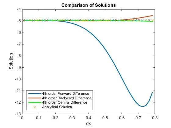
1. Comparison of solution

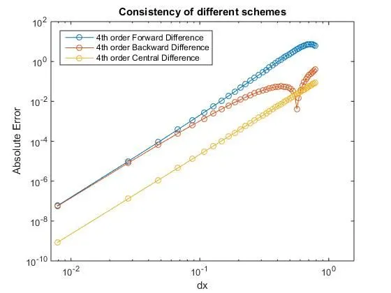
2. Comparison of absolute error

Conclusion

• From the first figure it is clear that all the numerical solutions are cconverging to the analytical solution as the grid size reduces. It is also noted that central differences scheme is converging to the solution at higher grid sizes also. Where as skewed schemes failed to converge to analytical solution at higher grid sizes.
• From the Second figureit is clear that the central scheme provides much more accurate solution as the absolute error is very small comprared with the skewed schemes.
• One remarkable use of skewed scheme is that it can be empolyed at the end nodes easily, where as the central scheme fails to apply at the end nodes.