Week 7 - Simulation of a 1D Super-sonic nozzle flow simulation using Macormack Method
AIM :
Simulate the isentropic flow through a quasi 1D subsonic-supersonic nozzle using the conservative and non-conservative forms of governing equations and solve them using the MacCormack's technique and compare the solutions of both the forms.
PROBLEM DEFINITION
A 1D converging - diverging nozzle (CD Nozzle) is used to solve the proble as shown in the figure.
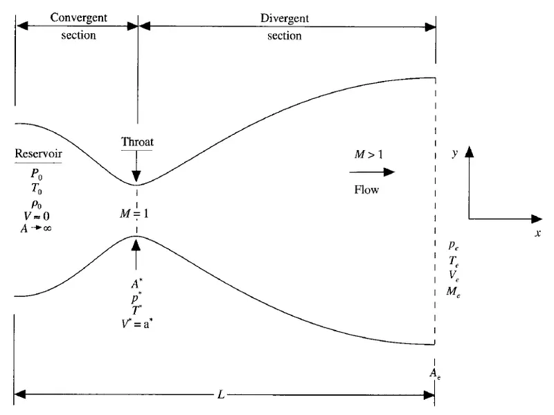
- It is assumed that there is only flow in x direction. The primitive variables are varying along the length of the nozzle as the flow occurs.
- The flow in the convergent area is always subsonic and the flow in the divergent area is supersonic.
- We are considering non-dimensionalied quanities for writing the governing equations and solving them.
The Governing equations in Non-conservative form are as follows
1. Continuity Equation.
`(delrho')/(delt') =-rho'(delv')/(delx')-rho'v'(dellnA')/(delx')-v'(delrho')/(delx')`
2. Momentum Equation
`(delv')/(delt') =-v'(delv')/(delx')-1/gamma((delT')/(delx')+(T')/(rho')(delrho')/(delx'))`
3. Energy Equation
`(delT')/(delt') =-v'(delT')/(delx')-(gamma-1)T'[(delv')/(delx')+v'(dellnA')/(delx')]`
Where `gamma=1.4`
- Shape of the Nozzle ( Area function )
`A'=1+2.2(x-1.5)^2`
- The initial condition for Non-conservative form at `t=0`;
`rho' = 1-0.3146x'`
`T' = 1-0.2314x'`
`v = (0.1+1.09x')T'^(1/2)`
- Mass flow rate `m'=rho'A'v'`
- Pressure `P'=rho'T'`
- Mach Number `M = (v')/sqrt(T')`
The Governing equations in Conservative form are as follows
1. Continuity Equation
`(delU_1)/(delt') = -(delF_1)/(delx')`
2. Momentum Equation
`(delU_2)/(delt') = -(delF_2)/(delx')+J_2`
3. Energy Equation
`(delU_3)/(delt') = -(delF_3)/(delx')`
Where;
`F_1,F_2,F_3` are the flux vectors`
`U_1,U_2,U_3` are the solution vectors and `J_2` is the source term
Defined as;
`U1 = rho'A'`
`U2=rho'A'v'`
`U3=rho'A'[(T')/(gamma-1) + (gamma)/2v'^2]`
`F_1 = U_2`
`F_2=(U_2^2)/(U_1)+(gamma-1)/gamma[U_3-gamma/2(U_2^2)/U_1]`
`F_3=(gamma(U_2U_3)/U_1) - gamma((gamma-1)/2)(U_2^3/u_1^2)`
`J_2 = 1/gammarho'T'(delA')/(delx')`
- Shape of the Nozzle ( Area function )
`A'=1+2.2(x-1.5)^2`
- The initial condition for Non-conservative form at `t=0`;
`rho'=1` for `0<=x'<=0.5`
`rho' = 1-0.366(x'-0.5)` for `0.5<=x'<=1.5`
`rho' = 0.634-0.3879(x'-1.5)` for `1.5<=x'<=3.5`
`T'=1` for `0<=x'<=0.5`
`T' = 1-0.167(x'-0.5)` for `0.5<=x'<=1.5`
`T' = 0.833-0.13507(x'-1.5)` for `1.5<=x'<=3.5`
- Density `rho'=U_1A'`
- Pressure `P' = rho'T'`
- Velocity `v'=U_2/U_1`
- Temperature `T'=(gamma-1)(U_3/U_1-gamma/2v^2)`
- Mach Number `M = (v')/sqrt(T')`
- Mass flow rate `m' =U_2`
Methodology
The Governing equations in both the forms are solved by Macormack Method uaing Time marching
Macormack Method: In this method the governing equations are solved in two steps; First step is called Predictor method and second step is called corrector method.
1. Predictor step: Here the equations are solved using forward difference method
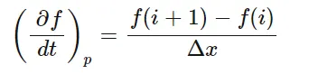
Solution Update: Here the solution is added with initial solutions and an updated solution is obtained.

2. Corrector Step: A backward differencing is carried out and asolution is obtained. Later an averaged result is obtaied by averaging predictor and corrector step.
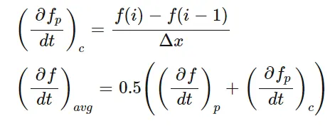
Final solution Update: Final solution is update itn this step

The following matlab code is used to solve this 1D subsonic-supersonic nozzle problem.:
Main Program:
% Simulation of a 1D Super-sonic nozzle flow simulation using Macormack Method

clc
clear all
close all

%  inputs, definig the spacial grid
n = [31 61];

gamma = 1.4;
C = 0.5;   % CFL number

% Time step
nt = 1:1400;
% dt = 0.01;

for nn = 1:length(n)

x = linspace(0,3,n(nn));

% Solving non-conservative equation
[m1,m1_throat,dt] = non_conservative(n(nn),nt,gamma,C);

% Soving conservative equation
[m2,m2_throat,dt] = conservative(n(nn),nt,gamma,C);

% Comparison of Normalized mass flow rate distributions of both forms
if n(nn)==31
figure(7)
subplot(2,1,1)
plot(nt,m1_throat,nt,m2_throat,'Linewidth',2)
title({['Mass flow rate distribution at throat'],['Non-conservative vs conservtive']})
legend('Non-conservative','Conservative')
xlabel('Timestep')
ylabel('Mass flow rate')

subplot(2,1,2)
plot(x,m1,x,m2,x,0.579,'*','Linewidth',2)
title({['Mass flow rate distribution in nozzle'],['Non-conservative vs conservtive']})
legend('Non-conservative','Conservative','Actual')
xlabel('Nozzle length')
ylabel('Mass flow rate')
end

% Grid independency test at throat
figure(8)
subplot(2,1,1)
plot(nt,m1_throat,'Linewidth',2)
xlabel('Timestep')
ylabel('Mass flow rate')
legend('31 nodes','61 nodes')
title('Conservative: Grid independency at throat')
hold on

subplot(2,1,2)
plot(nt,m2_throat,'Linewidth',2)
xlabel('Timestep')
ylabel('Mass flow rate')
legend('31 nodes','61 nodes')
title('Non-Conservative: Grid independency at throat')
hold on

end
Funcion file: Non-Conservative form:
function [m1,m1_throat,dt] = non_conservative(n,nt,gamma,C)

%  inputs defining spacial grid
x = linspace(0,3,n);
dx = x(2) - x(1);


% Initial connditions
rho = 1-0.3146*x;   % density
T = 1-0.2314*x;     % Temperature
v = (0.1+1.09*x).*T.^0.5; %Velocity

% Area profile
A = 1+2.2*(x-1.5).^2;  % Area

% Time loop
for i = 1:length(nt)

%     Defiining dt using CFL number
    for z=1:n
        dt(z) = C*dx/(sqrt(T(z))+v(z));
    end

    dt = min(dt);

    rho_old = rho;
    T_old = T;
    v_old = v;

    % Predictor step
    for j = 2:n-1

        % Forward differencing
        drho_dx = (rho(j+1)-rho(j))/dx;
        dv_dx = (v(j+1)-v(j))/dx;
        dlnA_dx = (log(A(j+1))-log(A(j)))/dx;
        dT_dx = (T(j+1)-T(j))/dx;

        % continuity equation
        drho_dt_p(j) = -rho(j)*dv_dx-rho(j)*v(j)*dlnA_dx-v(j)*drho_dx;

        % momentum equation
        dv_dt_p(j) = -v(j)*dv_dx-(1/gamma)*(dT_dx+(T(j)/rho(j))*drho_dx);

        % Energy equation
        dT_dt_p(j) = -v(j)*dT_dx - (gamma-1)*T(j)*(dv_dx+v(j)*dlnA_dx);

        % Solution updated
        rho(j) = rho(j) + drho_dt_p(j)*dt;
        v(j) = v(j) + dv_dt_p(j)*dt;
        T(j) = T(j) + dT_dt_p(j)*dt;
    end

    % corrector step
    for j = 2:n-1

        % Backward differencing
        drho_dx = (rho(j)-rho(j-1))/dx;
        dv_dx = (v(j)-v(j-1))/dx;
        dlnA_dx = (log(A(j))-log(A(j-1)))/dx;
        dT_dx = (T(j)-T(j-1))/dx;

        % continuity equation
        drho_dt_c(j) = -rho(j)*dv_dx-rho(j)*v(j)*dlnA_dx-v(j)*drho_dx;

        % momentum equation
        dv_dt_c(j) = -v(j)*dv_dx-1/gamma*(dT_dx+T(j)/rho(j)*drho_dx);

        % Energy equation
        dT_dt_c(j) = -v(j)*dT_dx - (gamma-1)*T(j)*(dv_dx+v(j)*dlnA_dx);

    end

        % Averaged solution
        drho_dt = 0.5*(drho_dt_p+drho_dt_c);
        dv_dt = 0.5*(dv_dt_p+dv_dt_c);
        dT_dt = 0.5*(dT_dt_p+dT_dt_c);

        % final solution update
        for k=2:n-1
        rho(k) = rho_old(k)+drho_dt(k)*dt;
        v(k) = v_old(k)+dv_dt(k)*dt;
        T(k) = T_old(k)+dT_dt(k)*dt;

        end

       % Pressure calculation
        P = rho.*T;

        % Mach number
        M = v./sqrt(T);

        % mass flow rate
        m1 = rho.*A.*v;

        % Applying new boundary conditions
        % inlet
        v(1) = 2*v(2)-v(3);

        % outlet
        v(n) =2*v(n-1) - v(n-2);
        rho(n) =2*rho(n-1) - rho(n-2);
        T(n) =2*T(n-1) - T(n-2);

        % Throat section properties
        rho_throat(i) = rho(16);
        v_throat(i) = v(16);
        T_throat(i) = T(16);
        P_throat(i) = P(16);
        M_throat(i) = M(16);
        m1_throat(i) = m1(16);

% Ploting mass flow rate at different timestep

if n==31
            if i == 1
            figure(1)
            plot(x,m1,'Linewidth',2)
            hold on
            elseif i==50
                plot(x,m1,'Linewidth',2)
            elseif i==200
                plot(x,m1,'Linewidth',2)
            elseif i==500
                plot(x,m1,'Linewidth',2)
            elseif i==1400
                plot(x,m1,'*','Linewidth',2)
                legend('nt=1','nt=50','nt=200','nt=500','nt=1400')
                title({['Variation of Mass flow rate distribution inside the nozzle at different'],['time steps during the time-marching process:Non-conservative']})
                xlabel('Length of Nozzle')
                ylabel('Mass Flow rate - Non dimensionalized')
            end
end

end
% Ploting distribution of primitive variable inside the nozzle
if n==31
    figure(2)
        plot(x,v,x,rho,x,T,x,P,x,M,x,m1,'Linewidth',2)
%       title(sprintf('Time step = %d',i))
        title('Distribution of primitive variables inside the Nozzle:Non-conservative')
        xlabel('Length of Nozzle')
        ylabel('Non-dimensionalised Variable')
        legend('Velocity','Density','Temperatture','Pressure','Mach Number','Mass flow rate','Location','northwest')

%  Variation of primitive parameters with Timestep
        figure(3)
        plot(nt,v_throat,nt,rho_throat,nt,T_throat,nt,P_throat,nt,M_throat,nt,m1_throat,'Linewidth',2)
        legend('Velocity','Density','Temperatture','Pressure','Mach Number','Mass flow rate','Location','northeast')
        title('Variation of primitive parameters with Timestep at throat:Non-Conservative')
        xlabel('Timestep')
        ylabel('Variable')
end
end
Function file: Conservative form:
function[m2,m2_throat,dt] = conservative(n,nt,gamma,C)

%  inputs defining spacial grid
x = linspace(0,3,n);
dx = x(2) - x(1);

% defininig area profile
A = 1+2.2.*(x-1.5).^2;  % Area

% Initial connditions
for nx=1:length(x)
    if x(nx)<=0.5
        rho(nx) = 1;
        T(nx) = 1;
    elseif (x(nx)>0.5) && (x(nx)<=1.5)
        rho(nx) = 1-(0.366*(x(nx)-0.5));
        T(nx) = 1- (0.167*(x(nx)-0.5));
    elseif (x(nx)>1.5) && (x(nx)<=3.5)
        rho(nx) = 0.634-(0.3879*(x(nx)-1.5));
        T(nx) = 0.833 - (0.3507*(x(nx)-1.5));
    end
end

v = 0.59./(rho.*A);

% Defining solution vectors
u1 = rho.*A;
u2 = rho.*A.*v;
u3 = rho.*A.*(T./(gamma-1) + (gamma./2.*v.^2));

%     Defiining dt using CFL number
for z=1:n
        dt(z) = C*dx/(sqrt(T(z))+v(z));
    end
     dt = min(dt);

% Time loop
for i = 1:length(nt)

    % Storing initial solutions
     u1_old = u1;
     u2_old = u2;
     u3_old = u3;

      % Defining Flux vectors
        f1 = u2;
        f2 = u2.^2./u1 + ((gamma-1)/gamma).*(u3-gamma./2*(u2.^2)./u1);
        f3 = (gamma*u2.*u3./u1) - (gamma*(gamma-1)/2)*(u2.^3./u1.^2);

     % du1/dt = -df1/dx
     % du2/dt = -df2/dx+j2
     % du3/dt = -df3/dx
     % j2 = 1/gamma*rho*T*dA_dx;

     % Predictor step
     for j = 2:n-1

        % Forward differencing
        df1_dx = (f1(j+1)-f1(j))/dx;
        df2_dx = (f2(j+1)-f2(j))/dx;
        df3_dx = (f3(j+1)-f3(j))/dx;
        dA_dx = (A(j+1)-A(j))/dx;

        % Source term
        j2_p(j) = 1./gamma*rho(j).*T(j).*dA_dx;

        % continuity equation
        du1_dt_p(j) = -df1_dx;

        % momentum equation
        du2_dt_p(j) = -df2_dx +j2_p(j);

        % Energy equation
        du3_dt_p(j) = -df3_dx;
%
        % updated solution vectors
        u1(j) = u1_old(j) + du1_dt_p(j)*dt;
        u2(j) = u2_old(j) + du2_dt_p(j)*dt;
        u3(j) = u3_old(j) + du3_dt_p(j)*dt;

        % Upfating the variables
        rho =   u1./A;
        v = u2./u1;
        T = (gamma-1).*(u3./u1-gamma./2*v.^2);

        % Updating flux terms
        f1 = u2;
        f2 = u2.^2./u1 + ((gamma-1)/gamma)*(u3-gamma./2*(u2.^2)./u1);
        f3 = (gamma*u2.*u3./u1) - (gamma*(gamma-1)/2)*(u2.^3./u1.^2);

     end

     % corrector step
     for j = 2:n-1

        % Backward differencing
        df1_dx = (f1(j)-f1(j-1))/dx;
        df2_dx = (f2(j)-f2(j-1))/dx;
        df3_dx = (f3(j)-f3(j-1))/dx;
        dA_dx = (A(j)-A(j-1))/dx;

        %Source term
        j2_c(j) = 1./gamma.*rho(j).*T(j).*dA_dx;

        % continuity equation
        du1_dt_c(j) = -df1_dx;

        % momentum equation
        du2_dt_c(j) = -df2_dx +j2_c(j);

        % Energy equation
        du3_dt_c(j) = -df3_dx;

     end

        % Averaged solution
        du1_dt = 0.5*(du1_dt_p+du1_dt_c);
        du2_dt = 0.5*(du2_dt_p+du2_dt_c);
        du3_dt = 0.5*(du3_dt_p+du3_dt_c);

        % final solution update
        for k=2:n-1
        u1(k) = u1_old(k)+du1_dt(k)*dt;
        u2(k) = u2_old(k)+du2_dt(k)*dt;
        u3(k) = u3_old(k)+du3_dt(k)*dt;
        end

        % Final variable update
        rho = u1./A;
        v = u2./u1;
        T = (gamma-1).*(u3./u1-gamma./2*v.^2);
        P = rho.*T;
        M = v./sqrt(T);
        m2 = u2;

        % Applying new boundary conditions
        % inlet
        u1(1) = A(1);
        u2(1) = 2*u2(2) - u2(3);
        u3(1) = u1(1)*(T(1)/(gamma-1) +gamma/2*v(1)^2);

        % outlet
        u1(n) = 2*u1(n-1) - u1(n-2);
        u2(n) = 2*u2(n-1) - u2(n-2);
        u3(n) = 2*u3(n-1) - u3(n-2);


        % Throat section properties
        rho_throat(i) = rho(16);
        v_throat(i) = v(16);
        T_throat(i) = T(16);
        P_throat(i) = P(16);
        M_throat(i) = M(16);
        m2_throat(i) = m2(16);

%   Ploting mass flow rate at different timestep

if n==31

        if i == 1
            figure(4)
            plot(x,m2)
            hold on
            elseif i==50
                plot(x,m2,'Linewidth',2)
            elseif i==200
                plot(x,m2,'Linewidth',2)
            elseif i==500
                plot(x,m2,'Linewidth',2)
            elseif i==1400
                plot(x,m2,'*')
                legend('nt=1','nt=50','nt=200','nt=500','nt=1400')
                title({['Variation of Mass flow rate distribution inside the nozzle at different'],['time steps during the time-marching process:Conservative']})
                xlabel('Length of Nozzle')
                ylabel('Mass Flow rate - Non dimensionalized')
            end
end
end
% Ploting distribution of primitive variable inside the nozzle
 if n==31
     figure(5)
        plot(x,v,x,rho,x,T,x,P,x,M,x,m2,'Linewidth',2)
%       title(sprintf('Time step = %d',i))
        title('Distribution of primitive variables inside the Nozzle:Conservative')
        xlabel('Length of Nozzle')
        ylabel('Non-dimensionalised Variable')
        legend('Velocity','Density','Temperatture','Pressure','Mach Number','Mass flow rate','Location','northwest')

% Variation of primitive parameters with Timestep
        figure(6)
        plot(nt,v_throat,nt,rho_throat,nt,T_throat,nt,P_throat,nt,M_throat,nt,m2_throat,'Linewidth',2)
        legend('Velocity','Density','Temperatture','Pressure','Mach Number','Mass flow rate','Location','northeast')
        title('Variation of primitive parameters with Timestepat throat:Conservative')
        xlabel('Timestep')
        ylabel('Variable')
 end

end
Results:
After executing the above program, following results were obltained.
1. Non-Conservative Form
- Figure (1):Distribution of primitive variables inside the nozzle
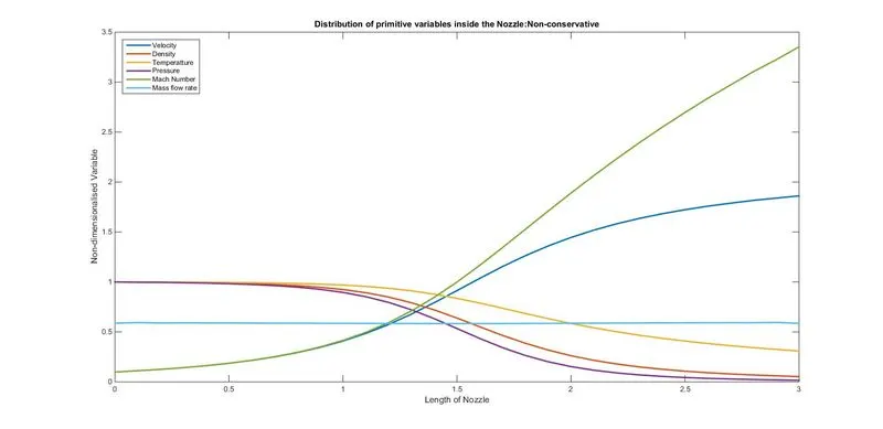
Figure 1 shows the variation of primitive parameters inside the nozzle. It is clear that the massflow rate is constant through out the length of the nozzle. Velocity is increasing as the flow continues its path. Simultaneously a supersonic flow (M>1) is observed at the nozzle exit. All the variables obtained are matching with the Anderson text data.
- Figure(2): Time-wise variation of primitive variables
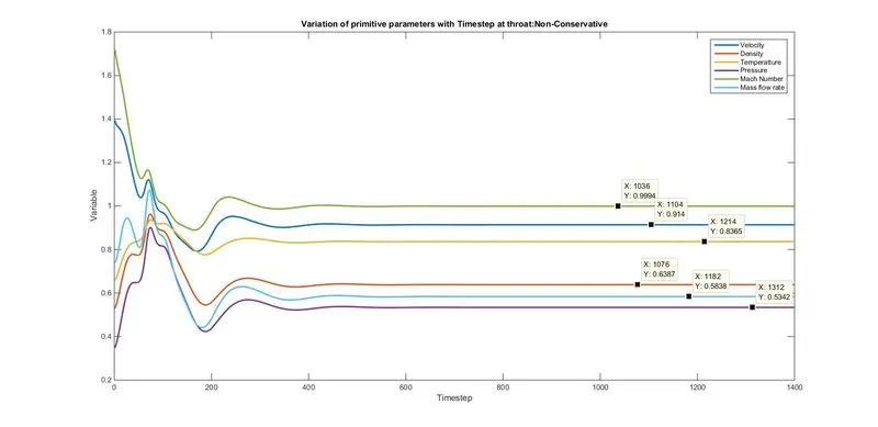
Figure(2) shows the time-wise variation of primitive variables at the throat section. It is clear from the graph that the variables are unstable during the initial timesteps and as the step increases it became stable. after 500 timesteps the parameters became very stable.
- Figure(3): Variation of Mass flow rate distribution inside the nozzle at different time steps during the time-marching process
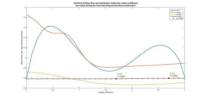
Figure(3) represents the variation of mass flow rate at different timesteps during the time-marching process. We can observe the mass flow rate at time steps 1,50,200, 500 and 1400. It is clear that after 500 timestep the mass flow rate is converging to a particular value. We can see that after 1400 steps the mass flow rate almost constant.
2. Conservative Form
- Figure(4): Distribution of primitive variables inside the nozzle
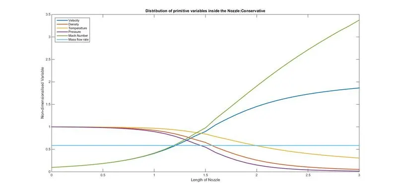
Figure(4) shows the variation of primitive parameters inside the nozzle. It is clear that the massflow rate is constant through out the length of the nozzle. Velocity is increasing as the flow continues its path. Simultaneously a supersonic flow (M>1) is observed at the nozzle exit. All the variables obtained are matching with the Anderson text data.
- Figure(5): Time-wise variation of primitive variables
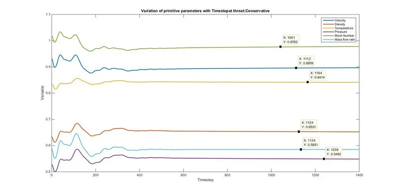
Figure(5) shows the time-wise variation of primitive variables at the throat section. It is clear from the graph that the variables are unstable during the initial timesteps and as the step increases it became stable. after 500 timesteps the parameters became very stable. The values are almost same as in Non-conervative form.
- Figure(6): Variation of Mass flow rate distribution inside the nozzle at different time steps during the time-marching process
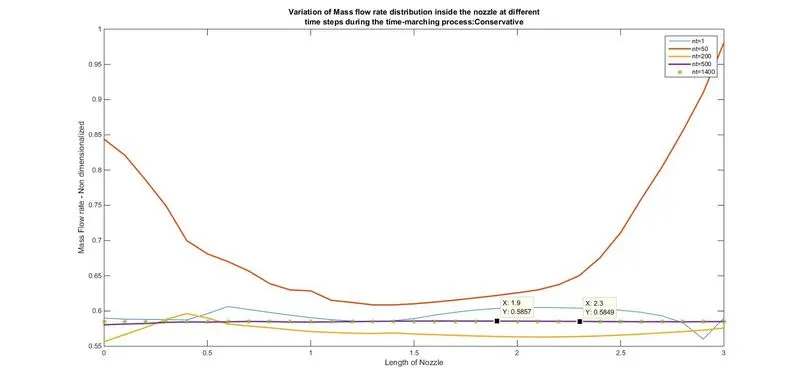
Figure(6) represents the variation of mass flow rate at different timesteps during the time-marching process. We can observe the mass flow rate at time steps 1,50,200, 500 and 1400. It is clear that after 500 timestep the mass flow rate is converging to a particular value. We can see that after 1400 steps the mass flow rate almost constant.
3. Comparison: Non-conservative vs Conservative form
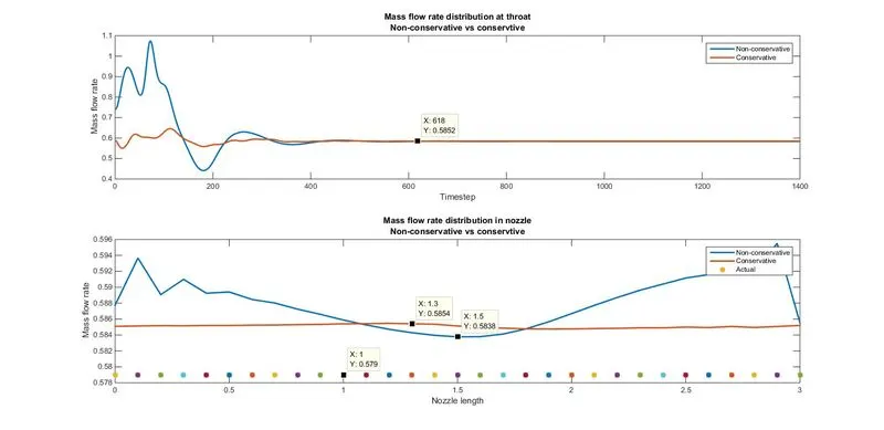
The above plot gives a comparison of non-conservative and conservative forms.
The first subplot campares the massflow rate at the throat at different timestep. Eventhough both forms converged to same stable solution, the Conservative form becomes stable faster than the Non-conservative form.
The second subplot compares the massflow rate though out the nozzle. We can observe that Conservative form is giving a constant massflow rate through out the nozzle.
4. Grid independence test on the solution
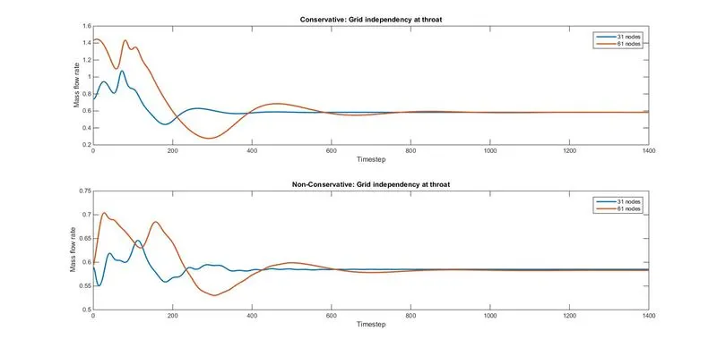
The above figure shows the grid independence test on the solution at the throat section. In both non conservative and conservative forms, lesser number of node gave a faster stable solution than higher number of nodes.
Conclusion
- From the study conducted above, it is clear that the Non-conservative as well as conservative forms of governing equation results almost same solutions.
- Both the form needs a minimum number of timestep to reach a stable solutions. At throat conservative form converged with lesser number of timesteps.
- Even after varying the number of nodes, alsmost same results were obtaned with less error.