Week 5.1 - Mid term project - Solving the steady and unsteady 2D heat conduction problem

Aim:

Solve the 2D steady and transient heat conduction equation using different iterative methods by using explicit and implicit form of equations and plot temperature contours.

The Boundary condition is as follows

Top Boundary = 600 K

Bottom Boundary = 900 K

Left Boundary = 400 K

Right Boundary = 800 K

Problem definition:

The general 2D heat conduction equation can be written as follows:

`(delT)/(delt) -alpha((del^2T)/(delx^2)+(del^2T)/(dely^2))=0`

The above equation can be solved in steady state and transient state.

1. Steady state: In steady state , we can assuming that time has no impact on the solution or the properties does not change with time. in other words,

`(delT)/(delt) = 0`

Therefore the steady state governing equation can be written as,

`(del^2T)/(delx^2)+(del^2T)/(dely^2) = 0`

2. Transient State: In transient state, the primitive variables changes as the time changes. Which means that time has impact on the solution. Therefore the governing equation can be written as,

`(delT)/(delt) -alpha((del^2T)/(delx^2)+(del^2T)/(dely^2))=0`

Methodology

These governing equations are solved using following iterative methods explicitly and implicitly as well.

• Jacobi method
• Gauss Siedel method (GS)
• Successive over relaxation (SOR)

In explicit form, there will be only one unknown inthe equations and the equations are not coupled, whereas in implicit form there will be multipled unknowns which are coupled with other equations.

1. Steady state

`(del^2T)/(delx^2)+(del^2T)/(dely^2) = 0`

The solution is,

`T_P = 1/k((T_L+T_R)/(delx^2)+(T_T+T_B)/(dely^2))`

where,

`T_P=T_(i,j)`

`T_L=T_(i-1,j)` & `T_R=T_(i+1,j)`

`T_B=T_(i,j-1)` & `T_T=T_(i,j+1)`

`k=2((delx^2+dely^2)/(delx^2dely^2))`

• Jacobi method : In Jacobi iterative method, the temperature in the `(n+1)^(th)`iteration is calculated from the temperature obtained from the old iteration ie. from `n^(th)` iteration.

`T_(P)=1/k((T_(L(old))+T_(R(old)))/(delx^2)+(T_(B(old))+T_(T(old)))/(dely^2))`

• Gauss Seidel method : In GS iterative method, the solver takes the temperature from `(n+1)^(th)`iteration to calculate the solution.

`T_(P)=1/k((T_(L)+T_(R(old)))/(delx^2)+(T_(B)+T_(T(old)))/(dely^2))`

• SOR method : It is an enhanced solver used to enhance the GS solver or Jacobi solver

`T_P=(1-omega)T_(P(old)) +omegaT_(GS)`

Where `omega` is relaxation factor taken as 1.2

2. Transient state Explicit

`(delT)/(delt) -alpha((del^2T)/(delx^2)+(del^2T)/(dely^2))=0`

the solution is given as

`T_P^(n+1)=T_P^n + k_1(T_R-2T_P+T_L)^n+k_2(T_T-2T_P+T_B)^n`

where `k_1=alpha(delt)/(delx^2)` & `k_2 = alpha(delt)/(dely^2)`

`alpha`= 1.4 = diffusion coeffiient

3. Transient State Implicit

The solution is given as,

`T_P^(n+1)=k[T_P^n + k_1(T_R+T_L)^(n+1)+k_2(T_T+T_B)^(n+1)]`

Where, `k=1/(1+2k_1+2k_2)`

The iterative concepts used in steady state is also used here.

The following codes are used to obtain the results for the above methodolgy.

Main program

1. Steady state solution.

% Mid term project - Solving the steady and unsteady 2D heat conduction problem
%  Top Boundary = 600 K
% Bottom Boundary = 900 K
% Left Boundary = 400 K
% Right Boundary = 800 K
% Steady state

clc
clear all
close all

nx = 21; % Number of x grid points
ny = nx; % Number of y grid points

x = linspace(0,1,nx);
y = linspace(0,1,ny);
dx = x(2)-x(1);
dy = y(2)-y(1);

k = 2*(((dx)^2+(dy)^2)/(dx*dy)^2);

omega = 1.2; % relaxation factor for SOR

tolerence = 1e-4;

[xx,yy] = meshgrid(x,y);

% defining temperature field
T = 300*ones(nx,ny);
T(1,:) = 600;
T(end,:) = 900;
T(:,1) = 400;
T(:,end) = 800;

% Storing initial temperature to Told
Told = T;


% Iterative solver 1 = Jacobi solver
% Iterative solver 2 = Gauss sieldel solver
% Iterative solver 3 = SOR solver

iterative_solver = 3;

% Solving 2D unsteady explicit system using Jacobi solver
if iterative_solver == 1
    iteration = 1;
    error = 9e9;
    while(error > tolerence)
         % Space loop
        for i =     2:nx-1
            for j = 2:ny-1
                TL = Told(i-1,j);
                TR = Told(i+1,j);
                TT = Told(i,j+1);
                TB = Told(i,j-1);
                T(i,j) = 1/k*((TL+TR)/(dx)^2 + (TT+TB)/(dy)^2);
                
            end
        end
        % Defining new error
        error = max(max(abs(Told - T)));
        % Updating temperature
        Told = T;
        iteration = iteration + 1        
       
    end
    % Jacobi Plot
     [x,y] = contourf(xx,yy,T);
        colormap(jet)
        colorbar
        clabel(x,y)
        title({['2D steady State conduction'],['Number of Jacobi Iteration =',sprintf('%d',iteration)]})
end

% Solving 2D unsteady explicit system using GS solver
if iterative_solver == 2
    iteration = 1;
     error = 9e9;
    while(error > tolerence)
        % Space loop     
        for i = 2:nx-1
            for j = 2:ny-1
                TL = T(i-1,j);
                TR = Told(i+1,j);
                TT = Told(i,j+1);
                TB = T(i,j-1);
                T(i,j) = 1/k*((TL+TR)/(dx)^2 + (TT+TB)/(dy)^2);
                
            end
        end
        % Defining new error
        error = max(max(abs(Told - T)));
        % Updating temperature
        Told = T;
        iteration = iteration + 1        
       
    end
    % GS plot
     [x,y] = contourf(xx,yy,T);
        colormap(jet)
        colorbar
        clabel(x,y)
        title({['2D steady State conduction'],['Number of GS Iteration =',sprintf('%d',iteration)]})
end
        
% Solving 2D unsteady explicit system using SOR solver               
 if iterative_solver == 3
    iteration = 1;
     error = 9e9;
    while(error > tolerence)
        % Space loop
        for i = 2:nx-1
            for j = 2:ny-1
                TL = T(i-1,j);
                TR = Told(i+1,j);
                TT = Told(i,j+1);
                TB = T(i,j-1);
                T(i,j) = Told(i,j)*(1-omega)+omega*(1/k*((TL+TR)/(dx)^2 + (TT+TB)/(dy)^2));
                
            end
        end
        % Defining new error
        error = max(max(abs(Told - T)));
        % Updating Temperature
        Told = T;
        iteration = iteration + 1      
       
    end
    % SOR plot
     [x,y] = contourf(xx,yy,T);
        colormap(jet)
        colorbar
        clabel(x,y)
        title({['2D steady State conduction'],['Number of SOR Iteration =',sprintf('%d',iteration)]})
end              

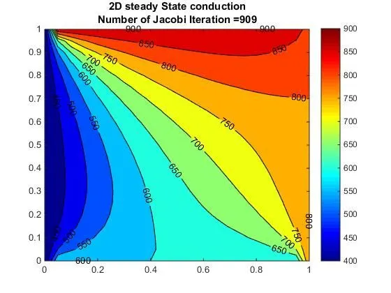
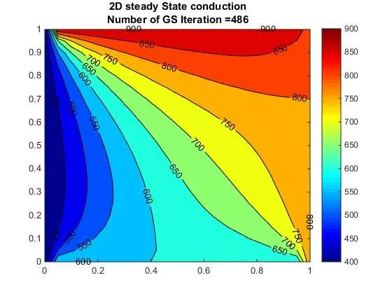
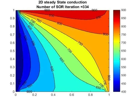
After executing the above code following results were obtained.

Observation

• From the above figures its is clear that all the three iterative solvers gave the same temperature distribution. Jacobi method needed 909 iterations to converge to the solution where as GS took 486 and SOR took 334 iterations. So it is clear that for steady state analysis SOR solver gives faster convergence compared to other two solvers.

2. Transient state Explicit form

% Mid term project - Solving the steady and unsteady 2D heat conduction problem
% Top Boundary = 600 K
% Bottom Boundary = 900 K
% Left Boundary = 400 K
% Right Boundary = 800 K
% Transient state Explicit.

clc
clear all
close all

nx = 21;  % Number of x grid points
ny = nx;  % Number of y grid points

x = linspace(0,1,nx);
y = linspace(0,1,ny);
dx = x(2)-x(1);
dy = y(2)-y(1);

omega = 1.2;   % relaxation factor for SOR
alpha = 1.4;   % diffusion coefficient

% Time step
dt = 0.5/((alpha/dx^2)+(alpha/dy^2));  % from stability criteria (cfl=0.5)
nt = 1000;


k1 = alpha*dt/(dx^2);
k2 = alpha*dt/(dy^2);

CFL = k1+k2;  % CFL number

K = 1+2*k1+2*k2;

tolerence = 1e-4;

[xx,yy] = meshgrid(x,y);

% defining temperature field
T = 300*ones(nx,ny);
T(1,:) = 600;
T(end,:) = 900;
T(:,1) = 400;
T(:,end) = 800;

% Storing initial temperature to Told
Told = T;

% Iterative solver 1 = Jacobi solver
% Iterative solver 2 = Gauss sieldel solver
% Iterative solver 3 = SOR solver

iterative_solver = 3;

% Solving 2D unsteady explicit system using Jacobi solver
    if iterative_solver == 1
   iteration = 1;   
   % Time loop
    for k = 1:nt       
      error = 9e9;  
    while(error > tolerence)
        % space loop
        for i = 2:nx-1
            for j = 2:ny-1
                TL = Told(i-1,j);
                TR = Told(i+1,j);
                TT = Told(i,j+1);
                TB = Told(i,j-1);
                term1 = Told(i,j);
                term2 = k1*(TR-2*Told(i,j)+TL);
                term3 = k2*(TT-2*Told(i,j)+TB);
                T(i,j) = term1+term2+term3;
                
            end
        end
        % defining new error
        error = max(max(abs(Told - T)));
        % updateing temperature
        Told = T;
        iteration = iteration + 1
    end       
    end
    % Jacobi plot
    figure(1)
        [x,y] = contourf(xx,yy,T);
        colormap(jet)
        colorbar
        clabel(x,y)
        title({['2D Transient explicit conduction'],['Number of Jacobi Iteration =',sprintf('%d',iteration)]})
    end
% Solving 2D unsteady explicit system using Gauss Siedel solver
if iterative_solver == 2
    iteration = 1;
    % Time loop
    for k = 1:nt
        error = 9e9;
    while(error > tolerence)
        % Space loop
        for i = 2:nx-1
            for j = 2:ny-1
                TL = T(i-1,j);
                TR = Told(i+1,j);
                TT = Told(i,j+1);
                TB = T(i,j-1);
                term1 = Told(i,j);
                term2 = k1*(TR-2*Told(i,j)+TL);
                term3 = k2*(TT-2*Told(i,j)+TB);
                T(i,j) = term1+term2+term3;
                
            end
        end
         % defining new error
       error = max(max(abs(Told - T)));
       % Updating temperature
       Told = T;
       iteration = iteration + 1
    end          
    end
    % Gauss Siedel plot
    figure(2)
        [x,y] = contourf(xx,yy,T);
        colormap(jet)
        colorbar
        clabel(x,y)
        title({['2D Transient explicit conduction'],['Number of GS Iteration =',sprintf('%d',iteration)]})
end  

% Solving 2D unsteady explicit system using SOR solver                
 if iterative_solver == 3
    iteration = 1;
    % Time loop
    for k = 1:nt
        error = 9e9;
    while(error > tolerence)
        % Space loop
        for i = 2:nx-1
            for j = 2:ny-1
                TL = T(i-1,j);
                TR = Told(i+1,j);
                TT = Told(i,j+1);
                TB = T(i,j-1);
                term1 = Told(i,j);
                term2 = k1*(TR-2*Told(i,j)+TL);
                term3 = k2*(TT-2*Told(i,j)+TB);
                T(i,j) = Told(i,j)*(1-omega)+omega*(term1+term2+term3);              
                
            end
        end
         % defining new error
        error = max(max(abs(Told - T)));
        % Updating temperature
        Told = T;
        iteration = iteration + 1
    end       
    end
    % SOR plot
    figure(3)
        [x,y] = contourf(xx,yy,T);
        colormap(jet)
        colorbar
        clabel(x,y)
        title({['2D Transient explicit conduction'],['Number of SOR Iteration =',sprintf('%d',iteration)]})
end

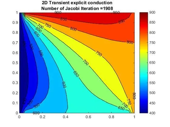
After executing the above code following results were obtained.

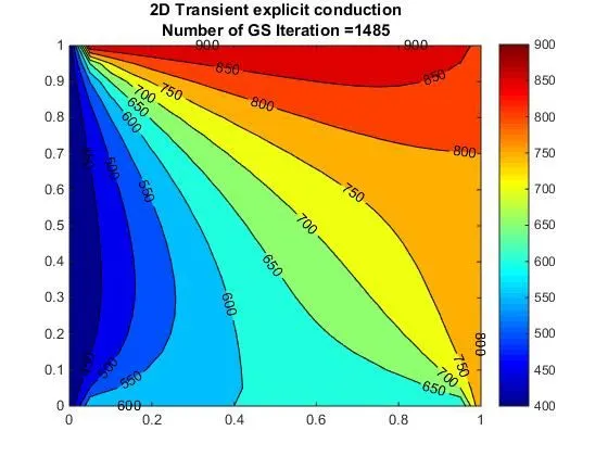
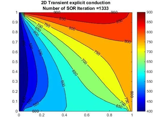
Observation

The above trend is repeated in transient explicit analysis also. The solution convergence rate is faster in SOR compared to all other solvers.

3. Transient State Implicit form

% Mid term project - Solving the steady and unsteady 2D heat conduction problem
% Top Boundary = 600 K
% Bottom Boundary = 900 K
% Left Boundary = 400 K
% Right Boundary = 800 K
% Transient state Implicit.

clc
clear all
close all

nx = 21; % Number of x grid points
ny = nx; % Number of y grid points

x = linspace(0,1,nx);
y = linspace(0,1,ny);
dx = x(2)-x(1);
dy = y(2)-y(1);

omega = 1.2;   % relaxation factor for SOR
alpha = 1.4;   % diffusion coefficient

% Time step
dt = 0.5/((alpha/dx^2)+(alpha/dy^2));  % from stability criteria (cfl=0.5)
nt = 1000;

k1 = alpha*dt/dx^2;
k2 = alpha*dt/dy^2;

CFL = k1+k2; % CFL number

tolerence = 1e-4;

[xx,yy] = meshgrid(x,y);

% defining temperature field
T = 300*ones(nx,ny);
T(1,:) = 600;
T(end,:) = 900;
T(:,1) = 400;
T(:,end) = 800;

% Storing initial temperature to Told and TP
Told = T;
TP = Told;

% Iterative solver 1 = Jacobi solver
% Iterative solver 2 = Gauss sieldel solver
% Iterative solver 3 = SOR solver

iterative_solver = 3;

% Solving 2D unsteady explicit system using Jacobi solver
if iterative_solver == 1
    iteration = 1;
    % Time loop
    for k = 1:nt
        error = 9e9;
    while(error > tolerence)
        % Space loop
        for i = 2:nx-1
            for j = 2:ny-1
                TL = Told(i-1,j);
                TR = Told(i+1,j);
                TT = Told(i,j+1);
                TB = Told(i,j-1);
                term1 = 1/(1+2*k1+2*k2);
                T(i,j) = term1*(TP(i,j)+k1*(TL+TR)+k2*(TT+TB));
                
            end
        end
        % Defining new error
        error = max(max(abs(Told - T)));
        % Updating Temperature
        Told = T;
        iteration = iteration + 1
    end
    % Updating previous Timestep Temperature
    TP = T;
       
    end
    % Jacobi Plot
     [x,y] = contourf(xx,yy,T);
        colormap(jet)
        colorbar
        clabel(x,y)
        title({['2D Transient Implicit conduction'],['Number of Jacobi Iteration =',sprintf('%d',iteration)]})
end

% Solving 2D unsteady explicit system using GS solver
if iterative_solver == 2
    iteration = 1;
    % Time loop
    for k = 1:nt
        error = 9e9;
    while(error > tolerence)
        % Space loop
        for i = 2:nx-1
            for j = 2:ny-1
                TL = T(i-1,j);
                TR = Told(i+1,j);
                TT = Told(i,j+1);
                TB = T(i,j-1);
                term1 = 1/(1+2*k1+2*k2);
                T(i,j) = term1*(TP(i,j)+k1*(TL+TR)+k2*(TT+TB));
                
            end
        end
        % Defining new error
        error = max(max(abs(Told - T)));
        % updating Temperature
        Told = T;
        iteration = iteration + 1
    end
    % Updating Previous timestep temperature
    TP = T;       
    end
    % GS plot
     [x,y] = contourf(xx,yy,T);
        colormap(jet)
        colorbar
        clabel(x,y)
        title({['2D Transient Implicit conduction'],['Number of GS Iteration =',sprintf('%d',iteration)]})
end
        
% Solving 2D unsteady explicit system using SOR solver                
 if iterative_solver == 3
    iteration = 1;
    % Time loop 
    for k = 1:nt
        error = 9e9;
    while(error > tolerence)
        % Space loop
        for i = 2:nx-1
            for j = 2:ny-1
                TL = T(i-1,j);
                TR = Told(i+1,j);
                TT = Told(i,j+1);
                TB = T(i,j-1);
                term1 = 1/(1+2*k1+2*k2);
                T(i,j) = Told(i,j)*(1-omega)+omega*(term1*(TP(i,j)+k1*(TL+TR)+k2*(TT+TB)));
                
            end
        end
        % Defining new error
        error = max(max(abs(Told - T)));
        % Updating temperature
        Told = T;
        iteration = iteration + 1
    end
    % Updating previous timestep temperature
    TP = T;       
    end
    % SOR plot
     [x,y] = contourf(xx,yy,T);
        colormap(jet)
        colorbar
        clabel(x,y)
        title({['2D Transient Implicit conduction'],['Number of SOR Iteration =',sprintf('%d',iteration)]})
%         pause(0.03)
end

After executing the above code following results were obtained.

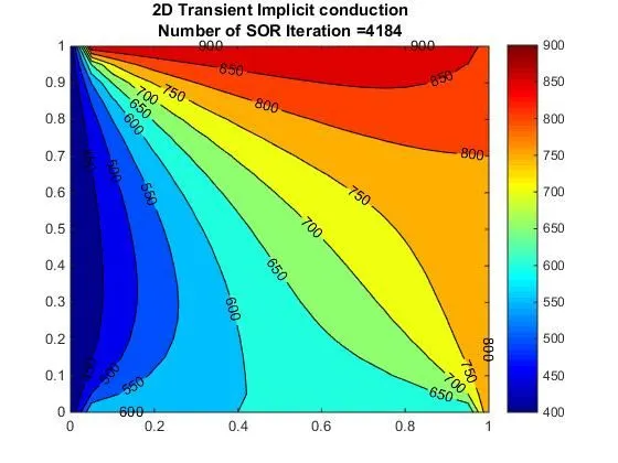
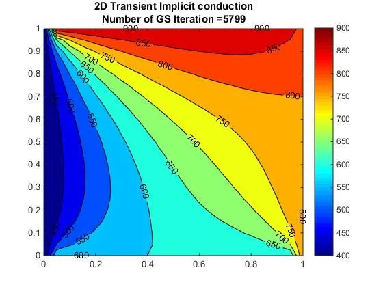
Observation

• The above trend is repeated in transient implicit analysis also. The solution convergence rate is faster in SOR compared to all other solvers.
• It is also noted that the implicit form took too much iterations to converge compared to explicit form.

Conclusions

• The steady state heat conducyion converges faster compared to the transient state.
• It is also noted that all the forms of governing equation pointing out to same solution regardless to the solver that is being used.
• It is also clear from the study that steady state solution converges very fast than the transient state.
• In all the analysis whether it is transient or steady, Jacobi solver takes too much of iterations and time to converge to a solution. Where as GS solver converges faster than the Jacobi. It is also noted that SOR is the fasted of all other solver depending upon the value of relaxation factor omega.
• So it is clear that SOR is the most effective solver compard to Jacobi and GS.
• In transient state analysis, the explit form arrives to solution very fast compared to implicit form.