Rayleigh Taylor Instability

Practical CFD models that are based on mathematical analysis of rayleigh Taylor waves:

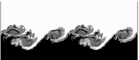
Kelvin–Helmholtz instability:

The theory predicts the onset of instability and transition to turbulent flow in fluids of different densities moving at various speeds. This instability occurs where there is a velocity shear or velocity difference between the interface of the two fluids.

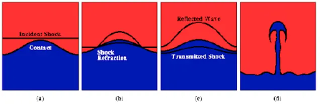
Richtmyer–Meshkov instability:

This type of instability occurs when there is an impulsive acceleration between two fluids. This type of instability can occur when there is a shock at greater speeds. The development of the instability begins with small amplitude perturbations which initially grow linearly with time. This is followed by a nonlinear regime with bubbles appearing in the case of a light fluid penetrating a heavy fluid and spikes appearing in the case of a heavy fluid penetrating a light fluid. A chaotic regime eventually is reached and the two fluids mix. This instability can be considered the impulsive-acceleration limit of the Ryleigh- Taylor instability.

Plateau–Rayleigh instability:

The Plateau–Rayleigh instability, often just called the Rayleigh instability, explains why and how a falling stream of fluid breaks up into smaller packets with the same volume but less surface area. It is related to the Ryleigh- Taylor instability. and is part of a greater branch of fluid dynamics concerned with fluid thread breakup. This fluid instability is exploited in the design of a particular type of inkjet technology. whereby a jet of liquid is perturbed into a steady stream of droplets. The driving force of the Plateau–Rayleigh instability is that liquids, by their surface tensions, tend to minimize their surface area. A considerable amount of work has been done recently on the final pinching profile by attacking it with self-similar solutions.

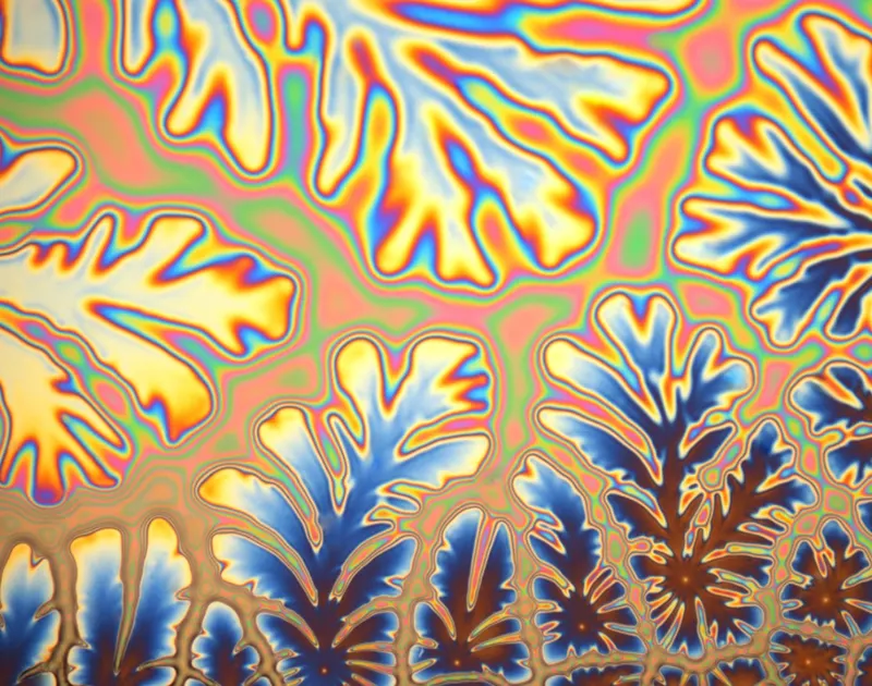
Saffman–Taylor instability:

The Saffman–Taylor instability, also known as viscous fingering, is the formation of patterns in a morphologically unstable interface between two fluids in a porous medium, described mathematically by Philip Saffman and G. I. Taylor in a paper of 1958. This situation is most often encountered during drainage processes through media such as soils. It occurs when a less viscous fluid is injected, displacing a more viscous fluid; in the inverse situation, with the more viscous displacing the other, the interface is stable and no instability is seen. Essentially the same effect occurs driven by gravity (without injection) if the interface is horizontal and separates two fluids of different densities, the heavier one being above the other: this is known as the Rayleigh-Taylor instability. In the rectangular configuration, the system evolves until a single finger (the Saffman–Taylor finger) forms, whilst in the radial configuration, the pattern grows to form fingers by successive tip-splitting.

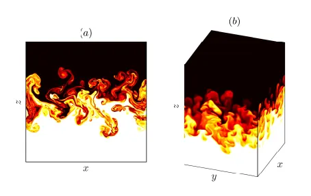
Rayleigh- Taylor instability simulation:

The Rayleigh–Taylor instability, or RT instability (after Lord Rayleigh and G. I. Taylor), is the instability of an interface between two fluids of different densities which occurs when the lighter fluid is pushing the heavier fluid. Examples include the behavior of water suspended above oil in the gravity of Earth, mushroom clouds like those from volcanic eruptions and atmospheric nuclear explosions, supernova explosions in which expanding core gas is accelerated into denser shell gas, instabilities in plasma fusion reactors, and inertial confinement fusion.

Visualization of an unstable Rayleigh–Taylor instability configuration where baroclinic torque at the interface creates vorticity and induces a velocity field that increases the baroclinic torque. Here ω is vorticity, p is pressure, ρ is density, u is velocity and g is gravity. The thick circular arrows represent the velocity field created by the vortex.

case 1 (Mesh size = 0.5)

Geometry:-

40*40 mm of two planes water and air heavier is above the lighter

The rayleigh Taylor instability occurs when two fluids' interface has different densities when the lighter fluid is pushing the heavier fluid. In this simulation, there are 2 surfaces Placed over each other. The geometry for the simulation is given below:

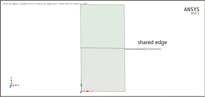
The upper square of the geometry represents water and the lower square represents air. The simulation is done for transient cases. At t= 0 the water in the above square is resting and the air in the lower square is also resting. As the simulation is carried out the water due to gravitational effects comes down and air moves up. During this process, there will be some instability that will occur at the surface. This simulation is performed to study the instabilities that occur at the interface.

Meshing:-

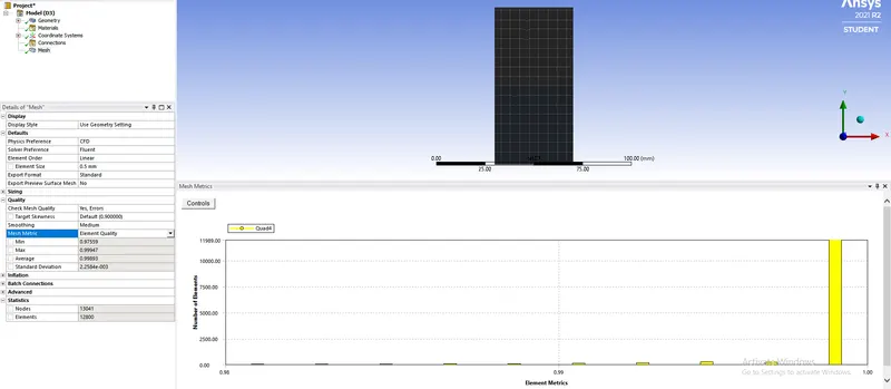
Mesh size = 0.5

Noodes = 13041

Elements =12800

Setup:-

The multiphase setup was used to study the instability. The method that was used to simulate the multiphase flow was the volume of liquids method.

Three cases of different mesh sizes were used to study the instability effects at the interface.

Solution Setup: -

case 1:-

1. General → Solver → Pressure-based → Time→ Transient → Gravity → 9.81m/s
2. Models →
3. Viscous → Laminar
4. Multiphase → Volume of fluid → 2 Eulerian Phase → Implicit Scheme

3. Material → Fluid → Add New → Fluent Database → water→copy→close
4. Method → Scheme → Simple
5. Initialize Solution → Standard
6. Results →
7. Create Contour → Phases → Volume Fraction → Field Variable = All Named Selections
8. Activities → Create Animation → Solution Animation → Phase Contour

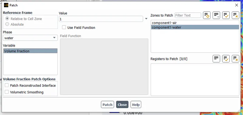
Patching should be done after every initialization

Results:-

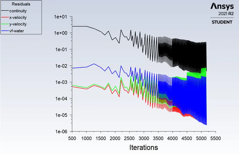
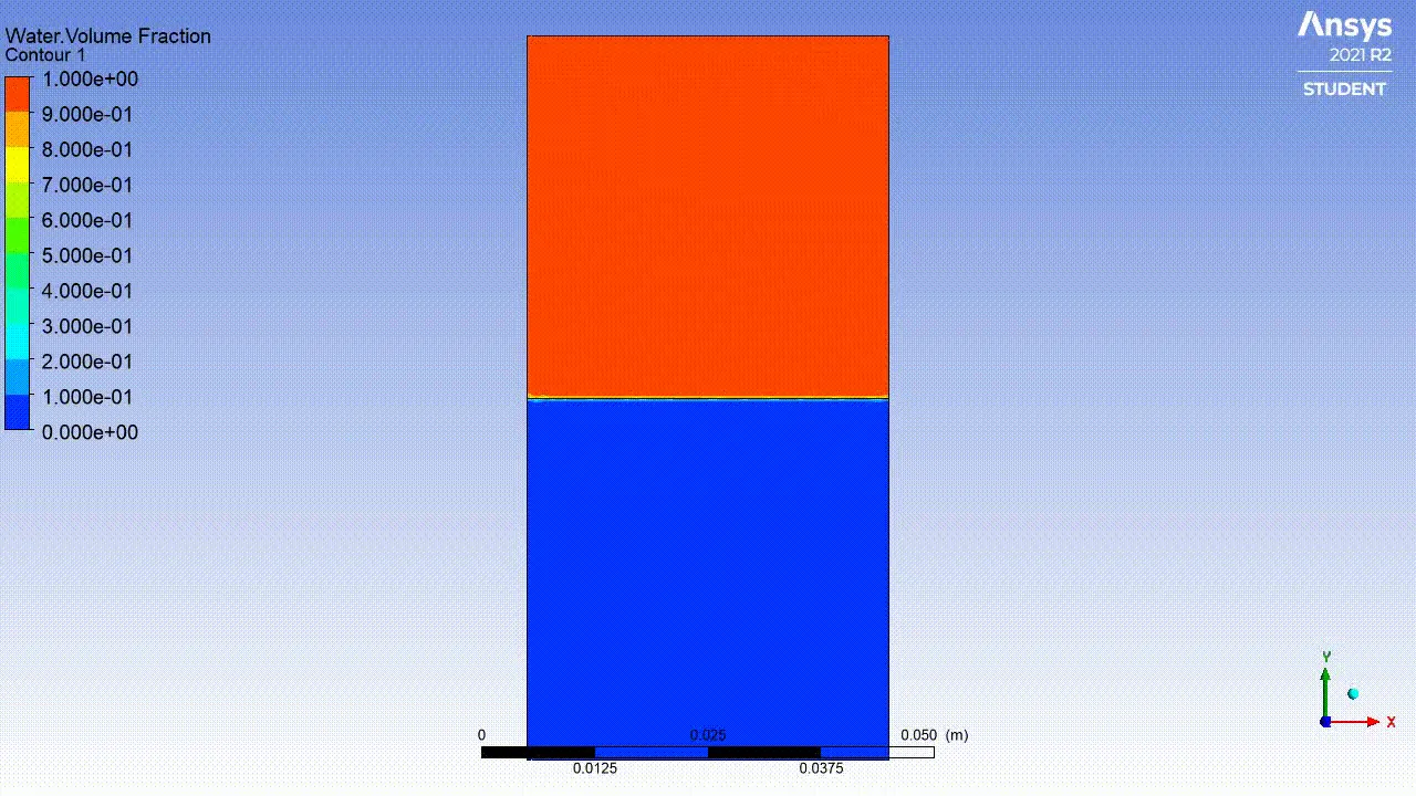
Case 1 (Refine mesh 0.2mm)

Mesh size = 0.2 mm

Noodes = 80601

Elements =80000

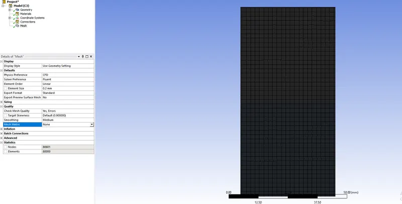
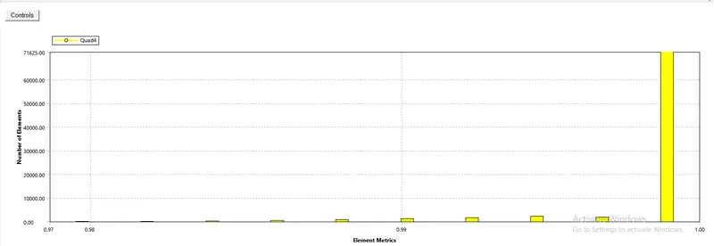
Mesh quality

Setup:-

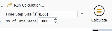
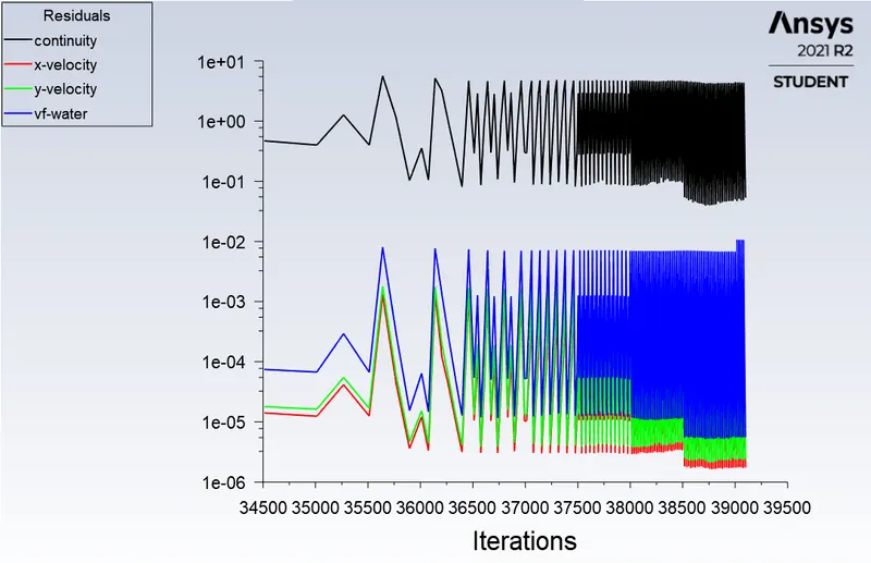
Time step size = 0.001 s

No.of Time steps = 2000

Results:-

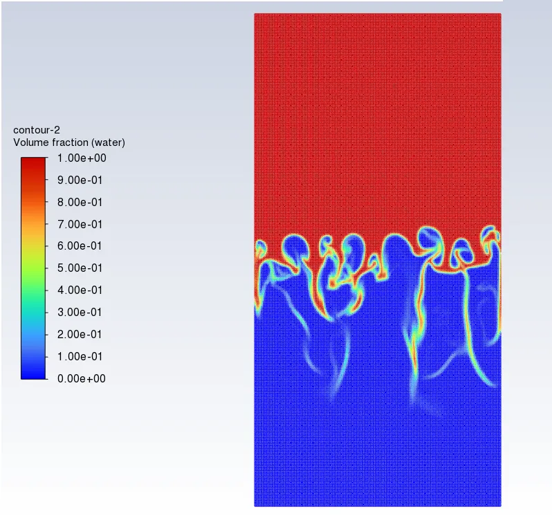
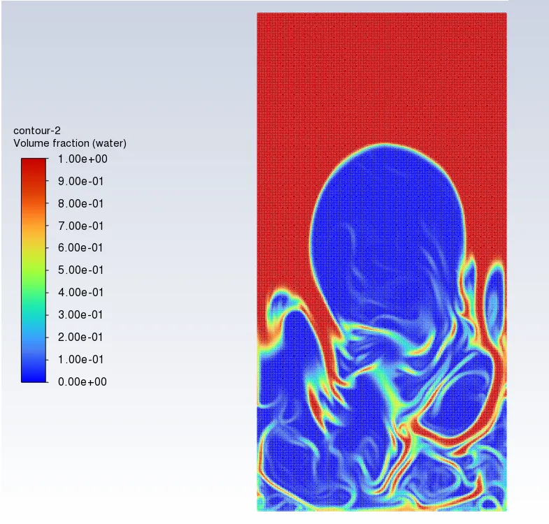
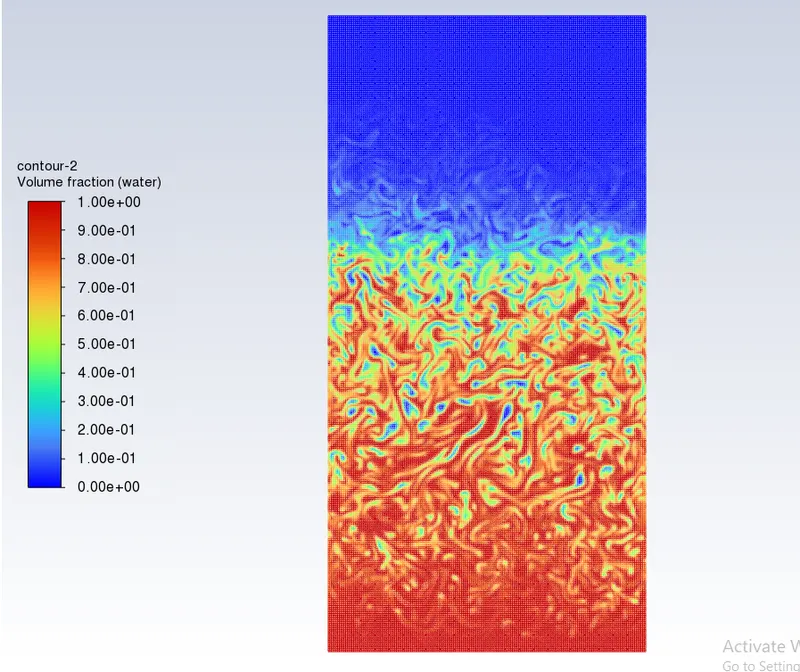
@time step 100 @time step 180 @time step 2000

case 2 :-

simulation with water and user-defined material(density = 400 kg/m³, viscosity = 0.001 kg/m-s) for refined mesh.

Setup:-

case 2 :-

1. General → Solver → Pressure-based → Time→ Transient → Gravity → 9.81m/s
2. Models →
3. Viscous → Laminar
4. Multiphase → Volume of fluid → 2 Eulerian Phase → Implicit Scheme

3. Material → Fluid → Add New → Fluent Database → User-Material (In our case user-material has Density=400 kg/m^3; viscosity = 0.001 kg/m-s)
4. Cell Zone Conditions → fff_surface → Fluid → User-material
5. Method → Scheme → Simple
6. Initialize Solution → Standard
7. Results →
8. Create Contour → Phases → Volume Fraction → Field Variable = All Named Selections
9. Activities → Create Animation → Solution Animation → Phase Contour

Time step size = 0.001 s

No.of Time steps = 2000

Results:-

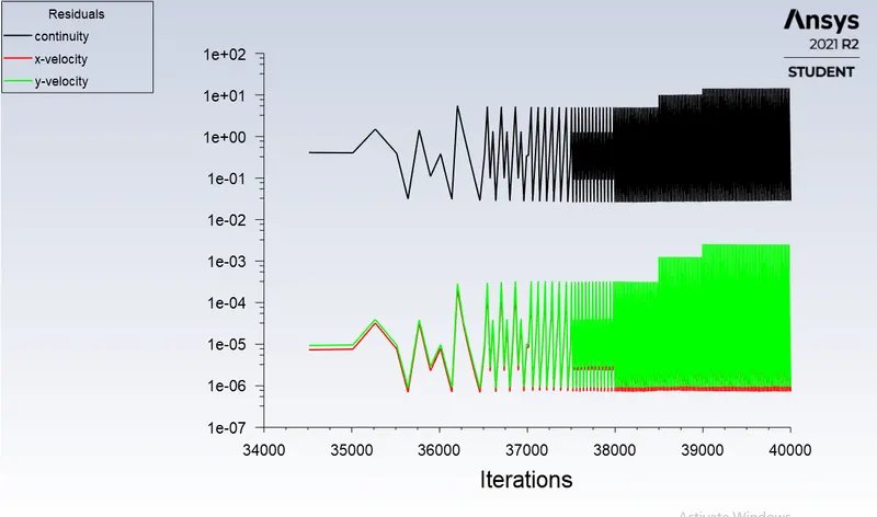
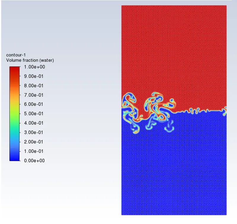
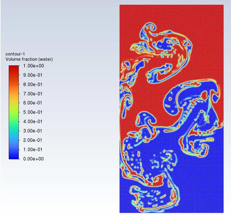
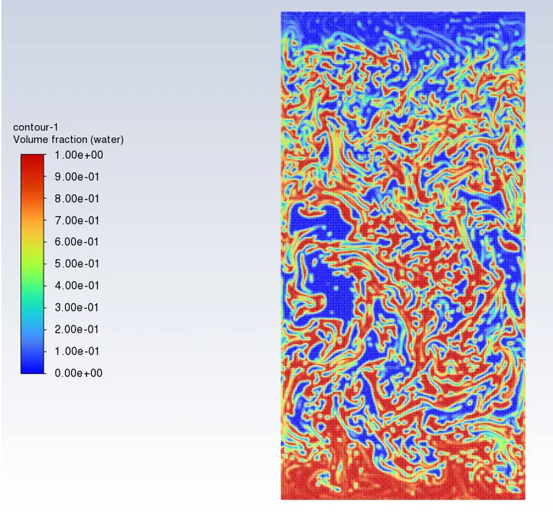
As we can see from the interface there are no large bubbles like plums because the user-defined density=400 is more compared to air so we can see this profile on initial

and the simulation should run for some more time to get settle

Observation -

For the above cases:

By comparing case 1 with two mesh sizes we can see that the computational time is more compared to mesh size 0.5 because elements in refine the mesh(0.2) are 6 times greater than the mesh size 0.5 and we can get more detailed profiles with the finer mesh(0.2), As we can see that there are large bubbles in case1 simulations

Compare to case 1(Refine mesh) and case2 time taken to get settled is more and we can see the different profiles

Atwood Number –

Atwood Number(A) is a dimensionless number in fluid dynamics used in the study of hydrodynamic instabilities in density stratified flows flow. It’s a dimensionless density ratio defined as:

`A=(ρ1−ρ2)/(ρ1+ρ2)`

Where,

`rho1`= density of the heavier fluid

`rho2`= density of the lighter fluid

Atwood number is an important parameter in the study of Rayleigh-Taylor instability and Richtmyer-Meshkov instability.

In Rayleigh-Taylor instability, the penetration distance of heavy fluid bubbles into the lighter fluid is a function of the acceleration time scale.

`A*g*t^2`

Where,

‘g’ is the acceleration due to gravity

‘t’ is time.

• For Atwood numbers close to 0, RT instability flows take the form of asymmetric “finger” of fluid.
• For Atwood number close to 1, the much lighter fluid “below” the heavier fluid takes the form of larger bubble-like plumes.
• Rayleigh-Taylor instability shows three distinct stag: Linear stability, Bubble formation(rising), and long-term evolution due to bubble merging and mixing.
• For low Atwood number, Bubble and Mushroom head shape is symmetrical, the disturbances or perturbations are linear for a large time.
• In contrast, Atwood number, Bubble and Mushroom head shape is asymmetrical.
• Also, it occurs at a rapid rate of acceleration which leads to a non-linear growth rate.

Case 1:

Heavier fluid (Water)

Density 1- 998.2 kg/m^3

Lighter Fluid (Air)

Density 2: 1.225 kg/m^3

Atwood number `A=(ρ1−ρ2)/(ρ1+ρ2)`

Atwood number(A)= 0.996

Case 2:

Heavier fluid (Water)

Density 1: 998.2 kg/m^3.

Lighter fluid (User-defined material)

Density 2: 400 kg/m^3

Atwood number `A=(ρ1−ρ2)/(ρ1+ρ2)`

Atwood number(A)= 0.4276

It’s observed from the simulation that air forms larger bubbles when water is burst down the air and forms large bubbles. The Atwood number calculated in case 1 and other cases = 0.42 (approx.).

Why steady-state approach might not be suitable for the above type of simulations?

• The difference between the steady and transient is that you can’t see the small variation of instability.
• The steady-state simulation is performed if we are more concerned about the final state or equilibrium state results.
• In RT- instability CFD models, we are interested in learning about the transition of irregularities that start developing when we pour high dense fluid upon low-density fluid under gravity effect so, by using a transient solver along with the refined mesh of the model.
• We can compute the smooth transition of irregularities that takes place at the interface of the fluids.
• The final state results for both the steady-state and transient state will be the same.
• Moreover, in the transient, we can see the behavior of the solution and every instant such that capturing Bubble, Vortex, and Shockwaves.

That’s the reason why transient is more suitable than the steady-state model.

Conclusion –

Rayleigh-Taylor instability simulation was studied at the interface of both fluids having different densities under the influence of gravity and the following observation were made:

• Finer mesh shows the formation of bubbles and vortices explicitly.
• Transient state analysis is preferred instead of steady-state analysis as we are interested in real-time changes at the interface.
• Atwood number depends on the density of the fluid and ranges from 0 to 1.
• Both Cases have larger Atwood numbers showing Rayleigh-Taylor instability. Hence matching the simulation results.