Week 5 - Rayleigh Taylor Instability
Objectives
- What are some practical CFD models that have been based on the mathematical analysis of Rayleigh Taylor waves? In your own words, explain how these mathematical models have been adapted for CFD calculations.
- Perform the Rayleigh Taylor instability simulation for 2 different mesh sizes with the base mesh being 0.5 mm. Compare the results by showing the animations( Attach them from your google drive). Observe the differences in the animation and explain the effect of mesh size on simulation. Also, explain why a steady-state approach might not be suitable for these types of simulation.[ Choose Air and Water for this simulation]
- Run one more simulation with water and user-defined material(density = 400 kg/m3, viscosity = 0.001 kg/m-s) for refined mesh.
- Define the Atwood Number. Find out the Atwood number for both the cases and explain how the variation in Atwood number in the above two cases affects the behavior of the instability.
Introduction
In numerous fields of study, the component of instability within a system is generally characterized by some of the outputs or internal states growing without bounds.Not all systems that are not stable are unstable; systems can also be marginally stable or exhibit limit cycle behavior
Fluid Instability
Fluid instabilities occur in liquids, gases and plasmas, and are often characterized by the shape that form; they are studied in fluid dynamics and magnetohydrodynamics. Fluid instabilities include
Kelvin–Helmholtz instability
This typically occurs when there is velocity shear in a single continues fluid, or additionally where there is a velocity difference across the interface between two fluids. A common example is seen when wind blows across a water surface; the instability constant manifests as waves. Kelvin-Helmholtz instabilities are also visible in the atmospheres of planets and moons, such as in cloud formations on Earth or the Red spot on Jupiter, and the atmospheres (coronas) of the Sun and other stars.
For a continuously varying distribution of density and velocity (with the lighter layers uppermost, so that the fluid is RT-stable), the dynamics of the Kelvin-Helmholtz instability is described by the Taylor Goldstein equation
Richtmyer–Meshkov instability (RMI)
It occurs when two fluids of different density are impulsively accelerated. Normally this is by the passage of a shock wave. The development of the instability begins with small amplitude perturbations which initially grow linearly with time. This is followed by a nonlinear regime with bubbles appearing in the case of a light fluid penetrating a heavy fluid, and with spikes appearing in the case of a heavy fluid penetrating a light fluid. A chaotic regime eventually is reached and the two fluids mix. This instability can be considered the impulsive-acceleration limit of the Rayleigh Taylor instability.
Plateau–Rayleigh instability,
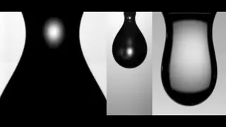
Is often just called the Rayleigh instability, explains why and how a falling stream of fluid breaks up into smaller packets with the same volume but less surface area. It is related to the Rayleigh taylor instability and is part of a greater branch of fluid dynamics concerned with fluid thread breakup. This fluid instability is exploited in the design of a particular type of ink jet technology whereby a jet of liquid is perturbed into a steady stream of droplets.
The driving force of the Plateau–Rayleigh instability is that liquids, by virtue of their surface tensions, tend to minimize their surface area. A considerable amount of work has been done recently on the final pinching profile by attacking it with self-similar solutions.[1][2]
Atwood Number
The Atwood number (A) is a dimensionless number in fluid dynamics used in the study of hydrodynamic instabilities in density stratified flows. It is a dimensionless density ratio defined as

where
 = density of heavier fluid
 = density of lighter fluid
Geometry
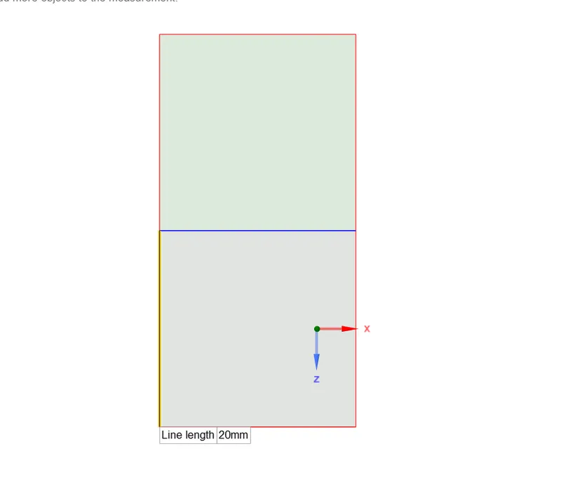
- Created two squares of 20mm one above the othre
Mesh
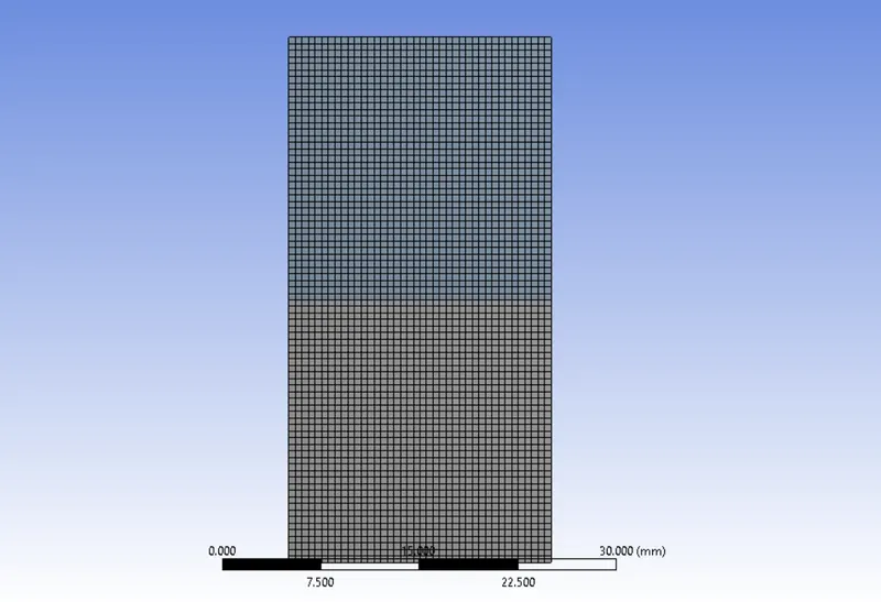
Case 1 (Base line mesh)
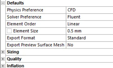
- Here I've used a mesh size of 0.5mm
Case 2 and Case 3(Refined mesh)
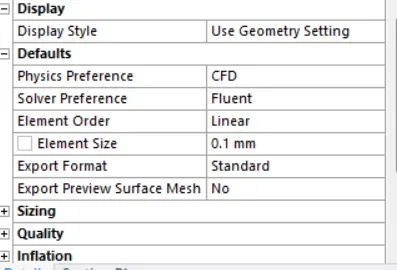
- Mesh size is set to 0.1 mm
Setup and Solution
Case 1
- Viscous model is set to Laminar
- A transient pressure based solver is used
- Gravity is turned on by setting 9.81m/s at negetive Y-axis
- Water is copied from Fluent database
- The two fluids were defined in Multiphase by selecting Volume of fluid and Implicit method is used
- And then the mesh geometry was checked to ensure the phases are located at desired locations
- Initialisation is done and then Patch option is used to define the Volume fraction of water in air(which is set to 0) and water(Set to 1)
- Contours of phases were defined and was recorded by using create animation tool
- Time step size is set to 0.005 and 1500 for number of time step
Solution
https://drive.google.com/file/d/10qkf-2jn-W5Pfl6TWd7mh7kaD4gnYJNh/view?usp=sharing
Case 2
- Viscous model is set to Laminar
- A transient pressure based solver is used
- Gravity is turned on by setting 9.81m/s at negetive Y-axis
- Water is copied from Fluent database
- The two fluids were defined in Multiphase by selecting Volume of fluid and Implicit method is used
- And then the mesh geometry was checked to ensure the phases are located at desired locations
- Initialisation is done and then Patch option is used to define the Volume fraction of water in air(which is set to 0) and water(Set to 1)
- Contours of phases were defined and was recorded by using create animation tool
- Time step size is set to 0.005 and 1500 for number of time step
Solution
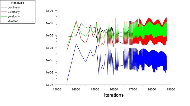
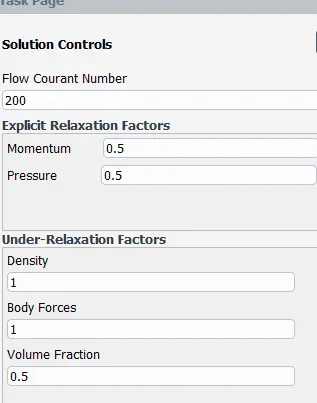
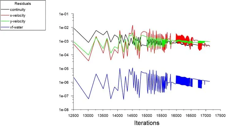
- A floating point error was found due to the divergance, Hence I've reduced the pressure and momentum values to 0.5 in solution control and the time step was increased to 0.01
https://drive.google.com/file/d/1P9q8dMXlKWKADlgD4UB97Q5P58AazQsI/view?usp=sharing
Case 3
- Viscous model is set to Laminar
- A transient pressure based solver is used
- Gravity is turned on by setting 9.81m/s at negetive Y-axis
- User defined material is defined as setting the density to 400 and viscosity to 0.001 and got it named as User defined 1
- The two fluids were defined in Multiphase by selecting Volume of fluid which is water and user defined fluid,and Implicit method is used
- And then the mesh geometry was checked to ensure the phases are located at desired locations (higher density at the top Initially)
- Initialisation is done and then Patch option is used to define the Volume fraction of water in Used defined fluid(which is set to 0) and in water ( is Set to 1)
- Contours of phases were defined and was recorded by using create animation tool
- Time step size is set to 0.005 and 1500 for number of time step
Solution
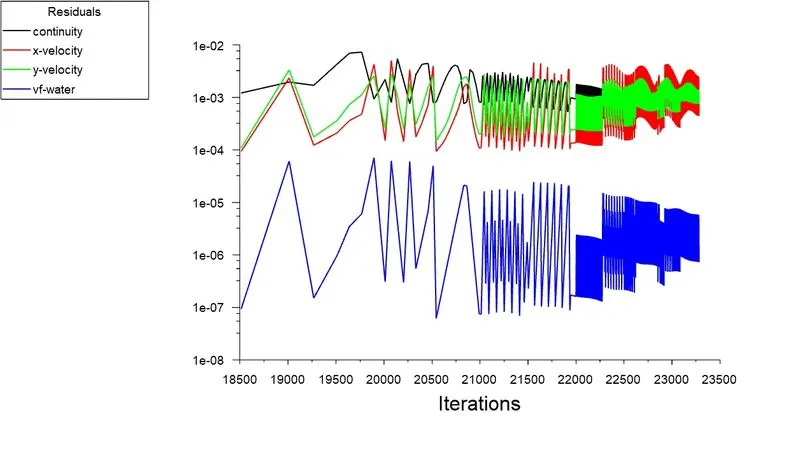
- A floating point error was found due to the divergance, Hence I've reduced the pressure and momentum values to 0.5 in solution control and the time step was increased to 0.01
https://drive.google.com/file/d/1OP8j4PKMIqAcl-z4SNej7SpAdGVaqkdK/view?usp=sharing
Atwood Number
- Atwood number for water and air = (1000-1.225)/(1000+1.225) = 0.9975
- Atwood number for water and user defined fluid = (1000-400)/(1000+400) = 0.4285
Why steady state analysis is not suitable for this simulation ?
The given case is time dependent which means at different time steps the phases are at different positions, So to observe the physical changes occuring in the simulation we need equations that carry time derivative terms , which is why I've selected transient case for this simulation
Observations
- When mesh was refined the difference in volume of water were much clear
- Refining mesh did involve floatation error due to divergance in which I had to reduce the pressure and momentum values in solution control
- Higher atwood number simulations shows faster mixing of phases and lower atwood number simulations seems the mixing of phases is slower
Conclusion
- Rayleigh taylor instability analysis was done on baseline mesh and on refined mesh
- Atwood number was calculated for both cases and behaviour of fluid mixing was analysed
- The simulation was done on water and a user defined fluid of density 400 kg/m^3 and of viscosity 0.001