Week 5 - Rayleigh Taylor Instability
AIM: To perform the Rayleigh Taylor Instability simulation for different mesh sizes.
Problem Statement:
- What are some practical CFD models that have been based on the mathematical analysis of Rayleigh Taylor waves? Explain how these mathematical models have been adapted for CFD calculations.
- Perform the Rayleigh Taylor instability simulation for different mesh sizes with the base mesh being 0.5 mm. Compare the results by showing the animations. Observe the differences in the animation and explain the effect of mesh size on simulation. Also, explain why a steady-state approach might not be suitable for these types of simulation.
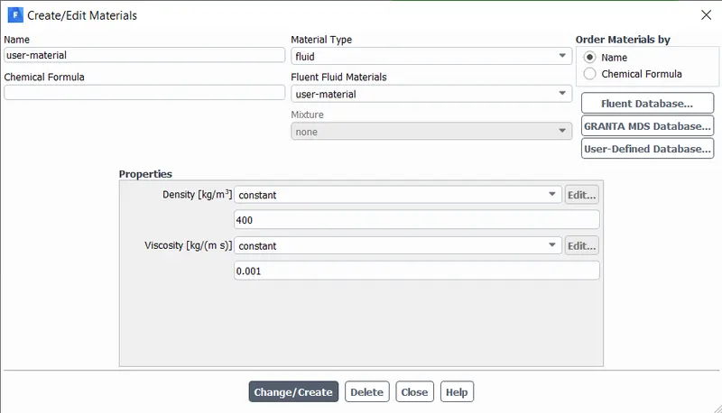
- Run one more simulation with water and user-defined material (density = `400 (kg)/m^3`, viscosity = `0.001 (kg)/(m s)`) for refined mesh.
- Define the Atwood Number. Find out the Atwood number for both the cases and explain how the variation in Atwood number in the above two cases affects the behavior of the instability.
THEORY:
Rayleigh-Taylor Instability:
The Rayleigh-Taylor instability is the instability of an interface between two fluids of different densities which occurs typically when the heavy fluid is supported by the lighter one. It may be modeled by two completely plane-parallel layers of immiscible fluid, the denser on top of the less dense one and both subject to the Earth's gravity. The equilibrium here is unstable to any perturbations or disturbances of the interface: if a parcel of heavier fluid is displaced downward with an equal volume of lighter fluid displaced upwards, the potential energy of the configuration is lower than the initial state. Thus the disturbance will grow and lead to a further release of potential energy, as the denser material moves down under the effective gravitational field and the less dense material is further displaced upwards. This was the set-up as studied by Lord Rayleigh. The important insight by G. I. Taylor was his realization that this situation is equivalent to the situation when the fluids are accelerated, with the less dense fluid accelerating into the more dense fluid. This occurs deep underwater on the surface of an expanding bubble and in a nuclear explosion.
As the RT instability develops, the initial perturbations progress from a linear growth phase into a non-linear growth phase, eventually developing plumes flowing upwards ( in the gravitational buoyancy sense ) and spikes falling downwards. In the linear phase, the fluid movement can be closely approximated by linear equations, and the amplitude of perturbations is growing exponentially with time. In the non-linear phase, perturbation amplitude is too large for a linear approximation, and non-linear equations are required to describe fluid motions.
In general, the density disparity between the fluids determines the structure of the subsequent non-linear RT instability flows (assuming other variables such as surface tension and viscosity are negligible here). The difference in the fluid densities divided by their sum is defined as the Atwood number, A. For A close to 0, RT instability flows take the form of symmetric "fingers" of fluid; for A close to 1, the much lighter fluid "below" the heavier fluid takes the form of larger bubble-like plumes.
Some CFD models that are based on the mathematical analysis of Rayleigh Taylor waves:
Kelvin-Helmholtz instability:
One of the most well-known instabilities in fluid mechanics is the instability at the interface between two horizontal parallel streams of different velocities and densities, with the heavier fluid at the bottom. This is called Kelvin-Helmholtz instability. The name is also commonly used to describe instability where the variations of velocity and density are continuous. The Kelvin-Helmholtz instability typically occurs when there is velocity shear in a single continuous fluid, or additionally where there is a velocity difference across the interface between two fluids. A common example is seen when the wind blows across a water surface; the instability constant manifests as waves. Kelvin-Helmholtz instabilities are also visible in the atmospheres of planets as moons, such as in cloud formations on Earth or the Red Spot on Jupiter, and the atmospheres of the Sun and other stars.
Plateau-Rayleigh instability:
A liquid jet, initially of constant radius, is falling vertically under gravity. The liquid length increases and reaches a critical value. At this critical value, the jet loses its cylindrical shape as it decomposes into a stream of droplets. This phenomenon occurs primarily as a result of surface tension. The driving force of the Plateau-Rayleigh instability is that liquids, by virtue of their surface tension, tend to minimize their surface area.
Joseph Plateau first characterized this instability through experimental observation, building on the work of Savart. He noted the inability arose when the liquid column length exceeded the column diameter by a factor of about 3.13. Lord Rayleigh later corroborated Plateau's work, giving an analytical explanation of this physical observation.
Richtmyer-Meshkov instability:
The Richtmyer-Meshkov instability (RMI) occurs when two fluids of different densities are impulsively accelerated. Normally this is by the passage of a shock wave. The development of instability begins with small amplitude perturbations which initially grow linearly with time. This is followed by a nonlinear regime with bubbles appearing in the case of a light fluid penetrating a heavy fluid, and with spikes appearing in the case of a heavy fluid penetrating a light fluid. A chaotic regime eventually is reached and the two fluids mix. This inability can be considered the impulsive-acceleration limit of the Rayleigh-Taylor instability.
During the implosion of an inertial confinement fusion target, the hot shell material surrounding the cold D-T fuel layer is shock-accelerated. This instability is also seen in magnetized target fusion. Mixing of the shell material and fuel is not desired and efforts are made to minimize any tiny imperfections or irregularities which will be magnified by RMI.
Salt fingering:
Salt fingering is a mixing process, the example of double-diffusive instability, that occurs when relatively warm, salty water overlies relatively colder, fresher water. It is driven by the fact that heated water diffuses more readily than salty water. A small parcel of warm, salty water sinking downwards into a colder, fresher region will lose its heat before losing its salt, making the parcel of water increasingly denser than the water around it and sinking further. Likewise, a small parcel of colder, fresher water will be displaced upward and gain heat by diffusion from surrounding water, which will then make it lighter than the surrounding waters, and cause it to rise further. Paradoxically, the fact the salinity diffuses less readily than the temperature means that salinity mixes more efficiently than temperature due to the turbulence caused by salt fingers.
Rayleigh-Taylor Instability simulation:
Steps involved:
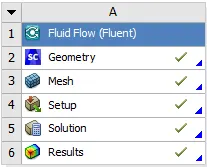
Geometry:
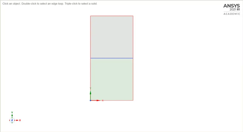
- Created a square of 20mm, and selected the pull tool to make it a surface of that.
- Created a new square of 20mm right on top of the first square which creates an interface between the two boxes.
- The upper square part is named water and the lower part is named air.
- The share topology is enabled to allow the flow of information through the interface between the fluids.
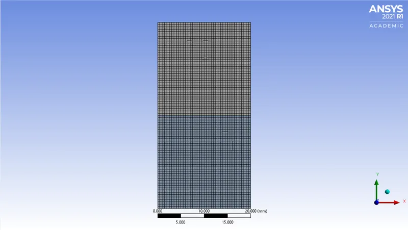
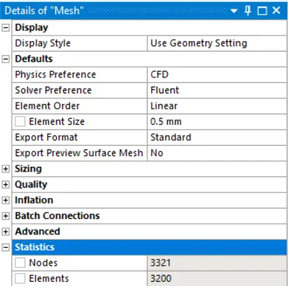
Mesh: After creating the geometry opened the mesh and generated the mesh with an element size of 0.5mm.
Case 1: Mesh element size: 0.5mm
Mesh:
Fluent setup:
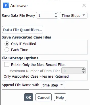
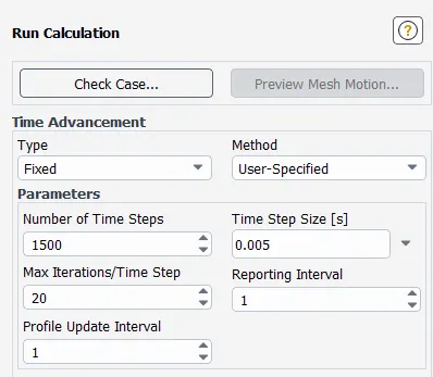
- After the meshing opened the fluent and set the general setting as shown below.
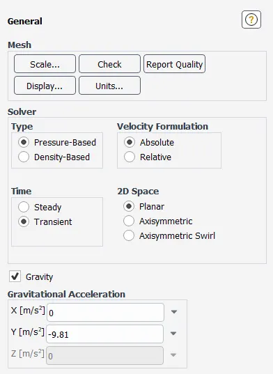
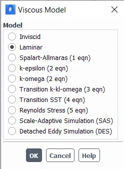
- Used Laminar Model
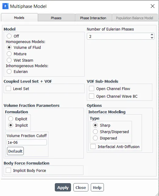
- Multiphase-->Model-->Volume of Fluid, Implicit Formulation
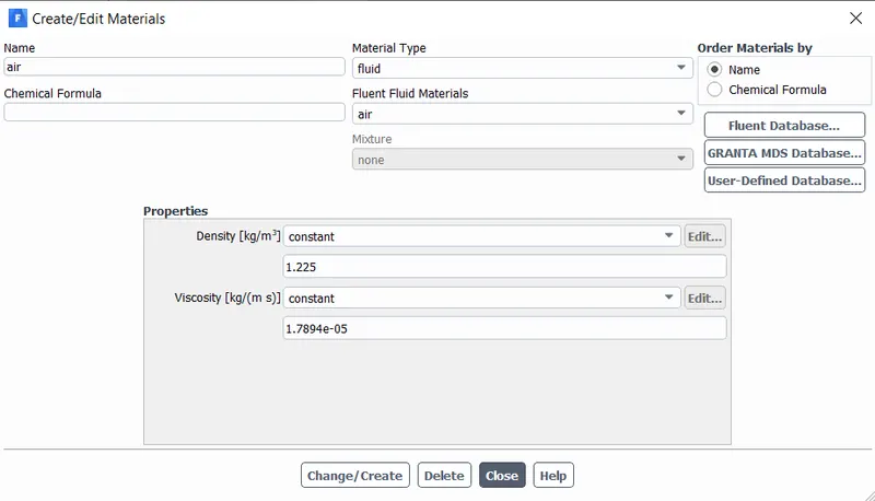
- Material selection--> Air and Water
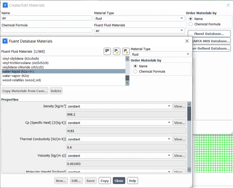
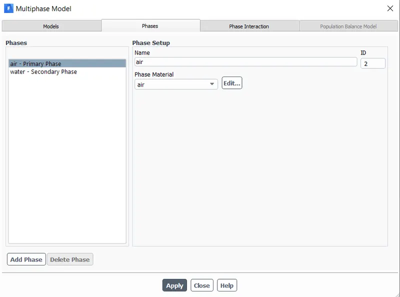
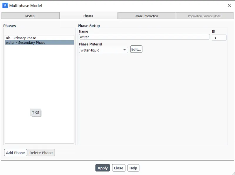
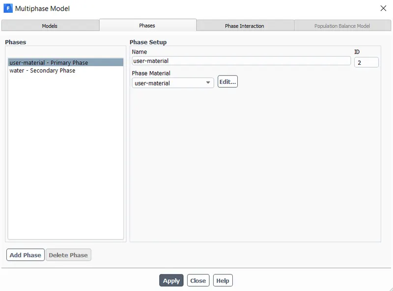
- Phases--> primary phase-Air, secondary phase-Water
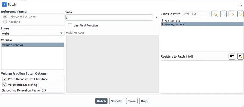
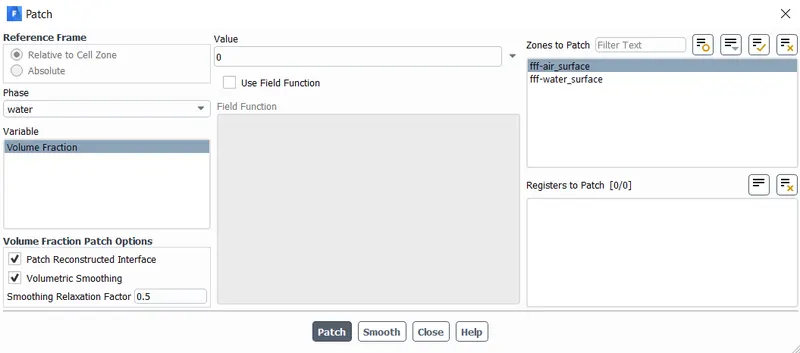
- Initialized using standard initialization, then used the patch option to give the value for water as 1 and 0 for air.
Residual plot:
Simulation animation:
Google drive link:
https://drive.google.com/file/d/1Zr8_n0zMiB4nCwKMLilbTQA3DafHCTs9/view?usp=sharing
Youtube link:
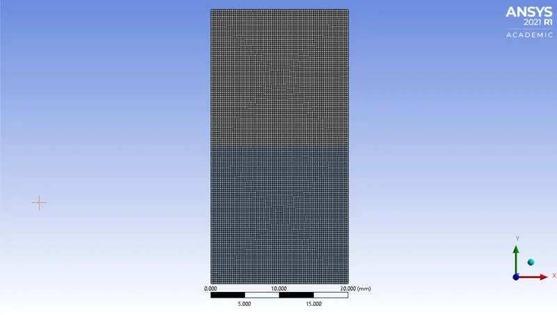
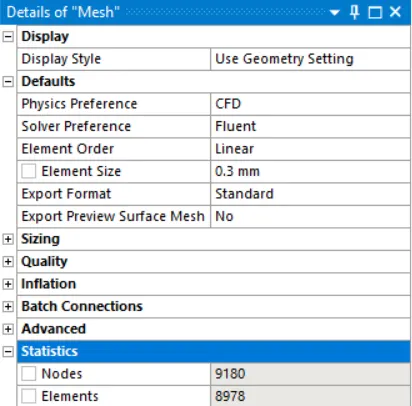
Case 2: Mesh element size: 0.3mm
Mesh:
Residual plot:
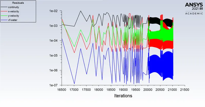
Simulation animation:
Google drive link:
https://drive.google.com/file/d/1CoF8Cp0E0GNgR0j9rfaUNBGFd7BNPz2j/view?usp=sharing
Youtube link:
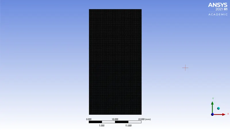
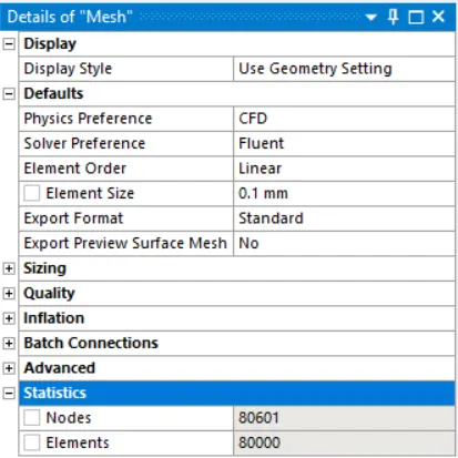
Case 3: Mesh element size: 0.1mm
Mesh:
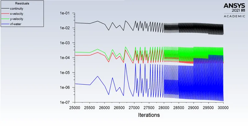
Residual plot:
Simulation animation:
Google drive link:
https://drive.google.com/file/d/1i_sbrAjXK8jmvaRlnLnNj2WGqSxdjzwe/view?usp=sharing
Youtube link:
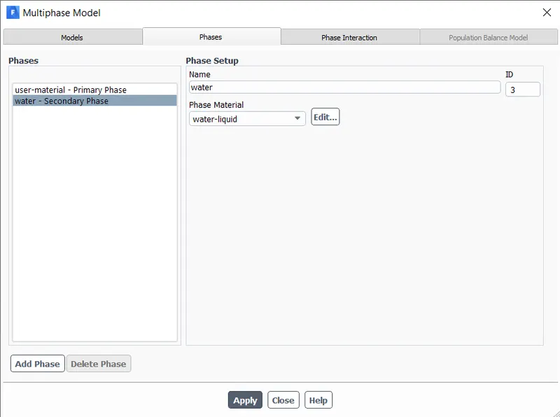
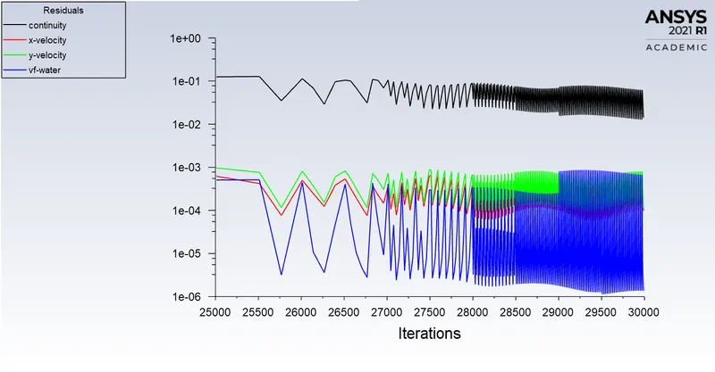
Case 4: Mesh element size: 0.1mm and having user-defined material and water
Mesh:
Residual plot:
Simulation animation:
Google drive link:
https://drive.google.com/file/d/1gmuqUuVCDPcpMUFqksMuDLvlEZthpp4R/view?usp=sharing
Youtube link:
Observations:
Effect of mesh size on simulation
Meshing has a direct influence on the accuracy and efficiency of CFD simulations. Once a meshing decision is made, it affects not only the types, numbers, orientation, and placement of grid elements, but also the simulation stability, convergence, and accuracy. The mesh generation process, therefore, plays a critical role in providing accurate, timely results.
It is observed that the more we refine the mesh, the more the simulation results get smoother about the irregularities that take place at the interface of the two fluids. As higher density fluid replaces the lower density fluid, the formation of air bubbles and vortex takes place, which travels towards the upward region with time.
In case 3, we can see the more detailed results about the formation of waves and the formation of some air bubbles that get trapped in the lower region during the initial stage and then they travel towards the upper region, generating shock waves. it is clearly visible because of the refined mesh.
At the end of the simulation, it is observed that the two phases get separated from each other, we can see some diffusivity between them which is a volume fraction of air and water.
We also observed as the mesh is refined further as in cases 2, 3, and 4 the computation time was relatively higher. We can say as we refine our mesh the computation time increases.
Why a steady-state approach might not be suitable for these types of simulations?
The steady-state simulation is performed if we are concerned more about the final state results or the equilibrium state. Steady-state is a state of the process which does not change with respect to time, we can't see the small-time variation of instability.
In our case Rayleigh Taylor instability CFD model, we are more concerned to learn about the transition of the irregularities that starts developing when we pour high dense fluid upon low dense fluid under the gravity effect, so by using transient simulation along with refined mesh we can compute the smooth transition of irregularities that takes place at the interface of the fluid.
In this problem, we are observing the instabilities when it is occurring so we are not concerned about the final answer. The final state results for both steady-state and transient states will be the same. The steady-state is more into capturing the final results nut by using transient we can see the behavior of the solution and every instant such that capturing bubbles, vortex, and shockwaves.
So this is the reason why transient is more suitable than steady-state simulation.
Atwood Number:
The Atwood number (A) is a dimensionless number in fluid dynamics used in the study of hydrodynamic instabilities in density stratified flows. It is a dimensionless density ratio. The difference in the fluid densities divided by their sum is defined as the Atwood number.
`A = (rho_1-rho_2)/(rho_1+rho_2)`
where
`rho_1 =` density of the heavier fluid
`rho_2=` density of the lighter fluid
Case 1: When water and air is used for simulation
The density of the heavier fluid (water), `rho_1` = `998.2 (kg)/m^3`
The density of the lighter fluid (air), `rho_2` = `1.225 (kg)/m^3`
Atwood number (A) = `(rho_1-rho_2)/(rho_1+rho_2)`
Atwood number (A) = 0.9975
Case 2: when water and user-defined material is used for simulation
The density of the heavier fluid (water), `rho_1` = `998.2 (kg)/m^3`
The density of the lighter fluid (user-defined material), `rho_2` = `400 (kg)/m^3`
Atwood number (A) = `(rho_1-rho_2)/(rho_1+rho_2)`
Atwood number (A) = 0.4278
For A close to 0, RT instability flows take the form of symmetric "fingers" of fluid; for A close to 1, the much lighter fluid "below" the heavier fluid takes the form of larger bubble-like plumes. This is how the Atwood number affects the behavior of the instability. It is seen from the simulation when water is poured down the air is pushed through and forms large bubbles for this case we got the Atwood number close to 1, and also the Atwood number closer to 1 signifies the same phenomenon which we have observed in our simulation.
Atwood number 0.4278 is close to 0. Hence, RT instability flows takes the form of symmetric "fingers" of fluid which can be observed from the animation video respectively. Hence this is the way we can validate our results.