Week 5: Prandtl Meyer Shock problem

PRANDTL MEYER SHOCK FLOW PROBLEM

Aim:-

The Prandtl Meyer shock flow is analysed with a subsonic and supersonic wave and the effect of SGS parameters in the problem.

Objective:-

• Run the Simulation with Subsonic(100m/s) and Supersonic(678m/s) waves.
• Varying the Sub-grid Criteria value in Adaptive mesh refinement to look at the effect of SGS temperature.
• Do a literature search on what BC's are typically used for shock flow problems.
• What is a shock wave? Describe the Physics behind shock waves.
• Show the mesh generation using Paraview.

Theory:-

Prandtl Meyer Shock Flow:-

A supersonic flow is expanded around a sharp expansion corner. An expansion wave is made up of an infinite number of Mach waves, diverging from a sharp corner. When a flow turns around a smooth and circular corner, these waves can be extended backwards to meet at a point.

Each wave in the expansion fan turns the flow gradually. It is physically impossible for the flow to turn through a single "shock" wave because this would violate the second law of thermodynamics.

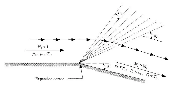
Across the expansion fan, the flow accelerates and the Mach number increases, while the static pressure, temperature and density decrease. Since the process is isentropic, the stagnation properties remain constant across the fan.

1. Literature search on what BC's are typically used for shock flow problems.

Types of boundary conditions:-

• Dirichlet boundary conditions.
• Neumann boundary conditions.
• Robin boundary conditions.
• Mixed boundary conditions.
• Cauchy boundary conditions.

The Dirichlet and Neumann boundary conditions are predominant. In the shock flow problem, the inlet boundary condition is Dirichlet and the outlet boundary condition is Neumann.

Dirichlet Boundary Condition:-

The Dirichlet boundary condition is imposed on an ordinary or a partial differential equation, it specifies the values that a solution needs to take along the boundary of the domain.

In Finite Element Method, Dirichlet boundary condition is defined by the weighted-integral form of a different equation. The dependent unknown u in the same form as the weight function w appearing in the boundary expression is termed a primary variable and its specification constitutes the Dirichlet boundary condition.

In fluid dynamics, the no-slip condition for viscous fluids states that at a solid boundary, the fluid will have zero velocity relative to the boundary.

Neumann Boundary Condition:-

The Neumann boundary condition is a type of boundary condition, named after Carl Neumann. When imposed on an ordinary or a partial differential equation, the condition specifies the value of the derivative applied at the boundary of the domain.

It is possible to describe the problem using other boundary conditions: a Dirichlet boundary condition specifies the value of the solution itself on the boundary, whereas the Cauchy boundary condition, mixed boundary conditions and Robin boundary condition are all different types of combinations of the Neumann and Dirichlet boundary conditions.

2. What is a Shock wave?

Shock waves are formed when a pressure front moves at supersonic speed and pushes on the surrounding air.

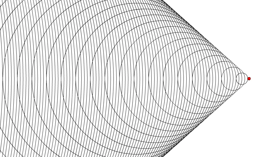
When the speed of the object exceeds the speed of the sound, the wavefronts lag behind the source in a cone-shaped region with the source at the vertex. The edge of the cone forms a supersonic wave with a large amplitude called a "shock wave". when a shock wave reaches an observer a "sonic boom" is heard.

In a shock wave, the properties of the fluid (density, pressure, temperature, flow velocity, Mach number) change almost instantaneously.

SIMULATION PROCESS

Part 1 - Subsonic condition (velocity 100 m/s)

• SGS temperature of 0.05 K
• SGS temperature of 0.025 K
• SGS temperature of 0.01 K

Part 2 - Supersonic condition (velocity 678 m/s)

• SGS temperature of 0.05 K
• SGS temperature of 0.025 K
• SGS temperature of 0.01 K

A. Geometry setup:-

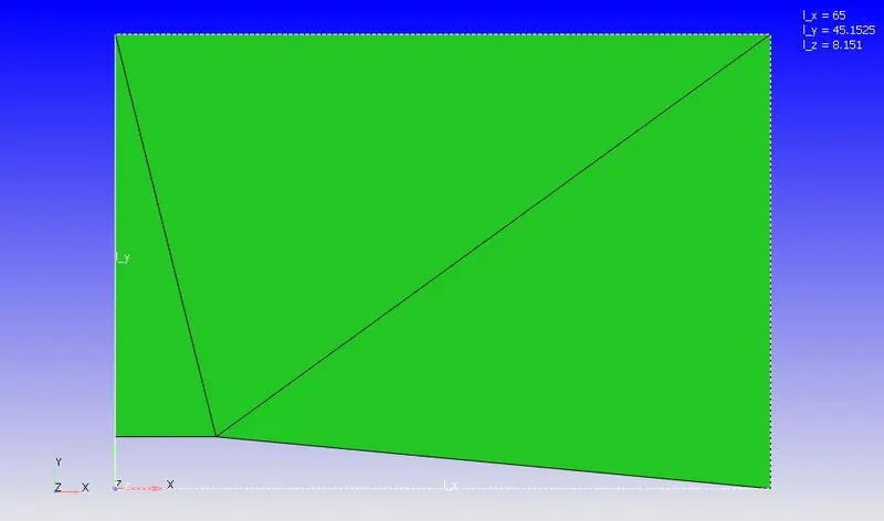
• Import the 2D supersonic flow.STL file in converge studio.
• Scale the geometry from millimeter to meter.
• Change the normals to the fluid flow direction.

Geometry:-

Boundary Flagging:-

B. Case Setup:-

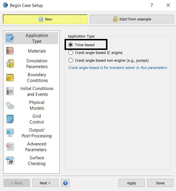
1. Application Type:-

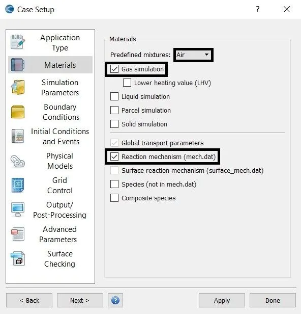
2. Material:-

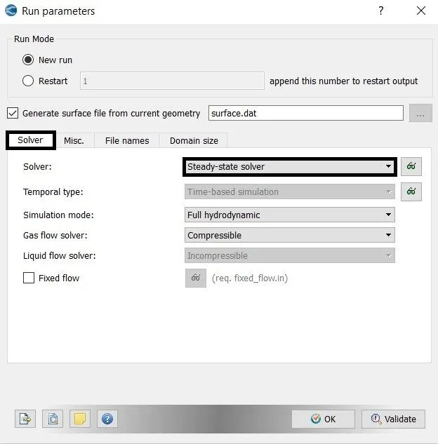
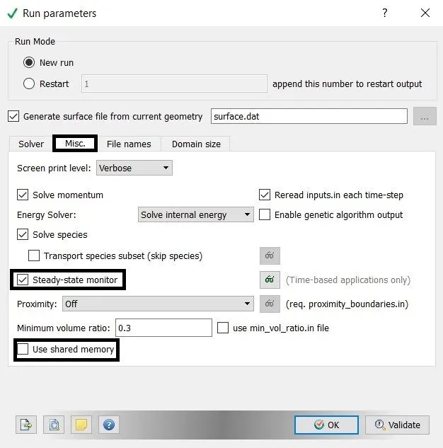
3. Simulation Parameters:-

• A steady-state solver is used.
• The steady-state monitor is enabled.
• Use share memory is disabled.

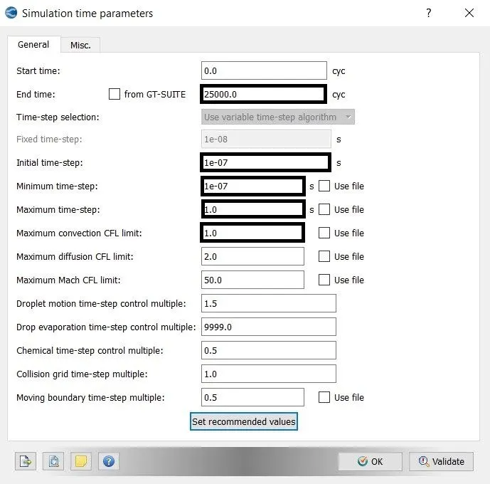
4. Simulation Time Parameters:-

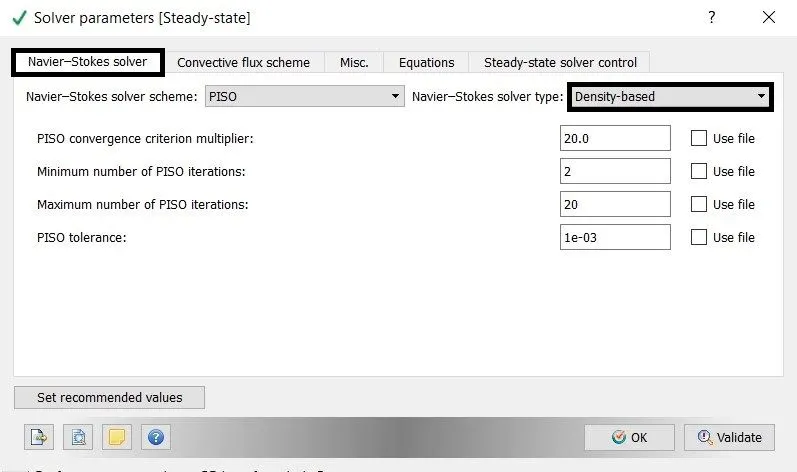
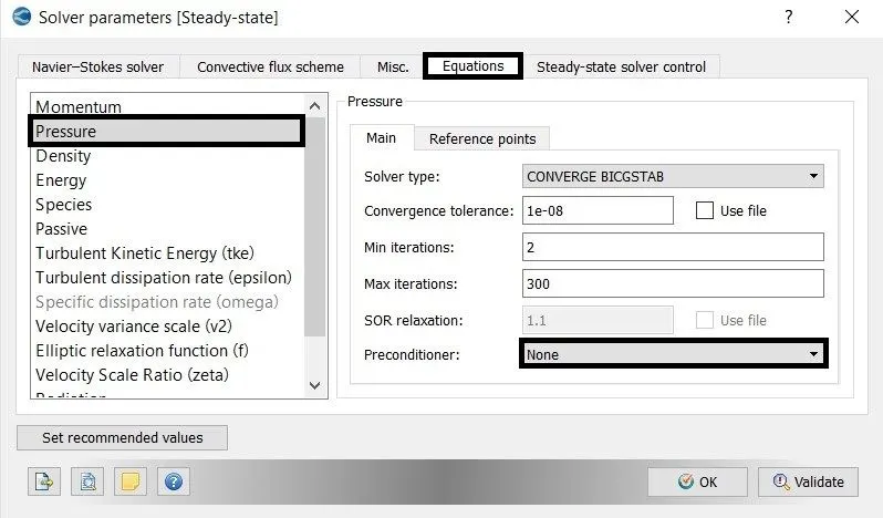
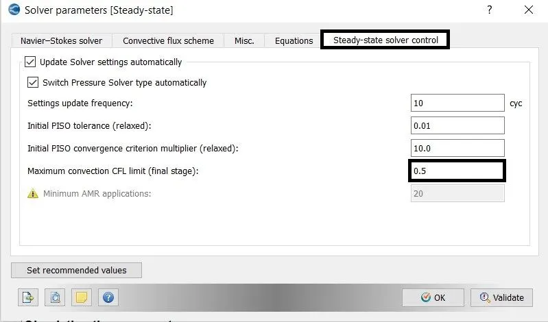
5. Solver Parameters:-

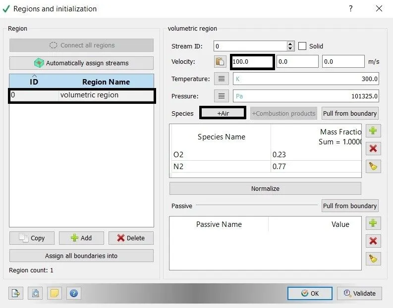
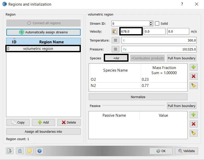
6. Region and Initialization:-

• Subsonic flow condition (velocity x = 100 m/s)
• Supersonic flow condition (velocity x = 678 m/s)

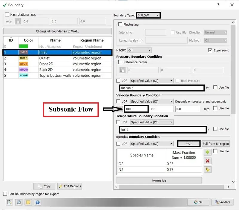
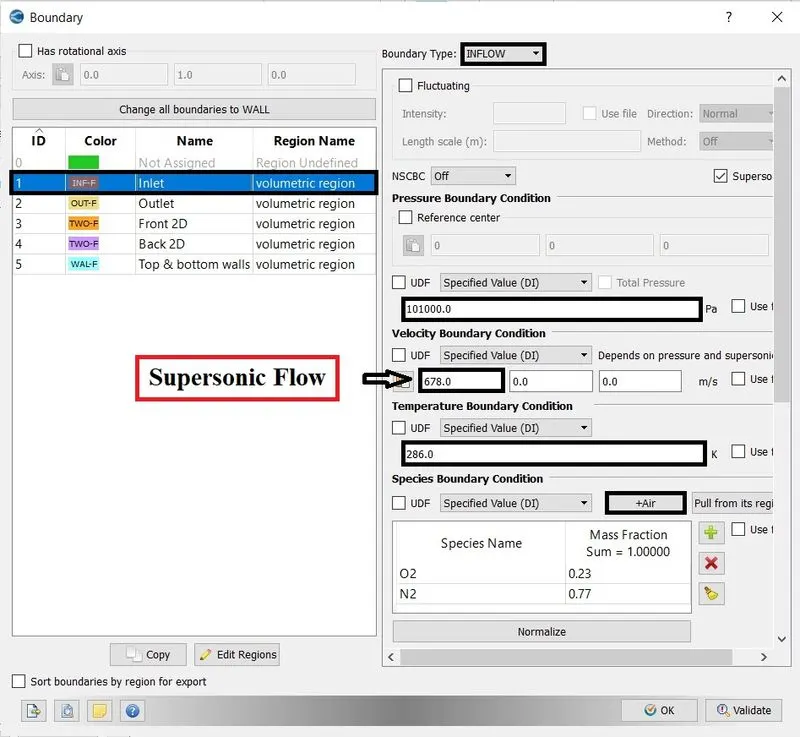
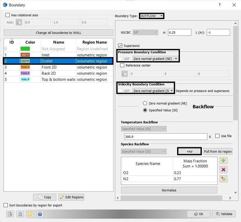
7. Boundary Condition:-

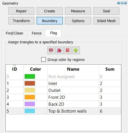
• Inlet = Dirichlet boundary condition
• outlet = Neumann boundary condition
• Front 2D = Two_D
• Back 2D = Two_D
• Top & Bottom walls = Wall with Slip boundary condition.

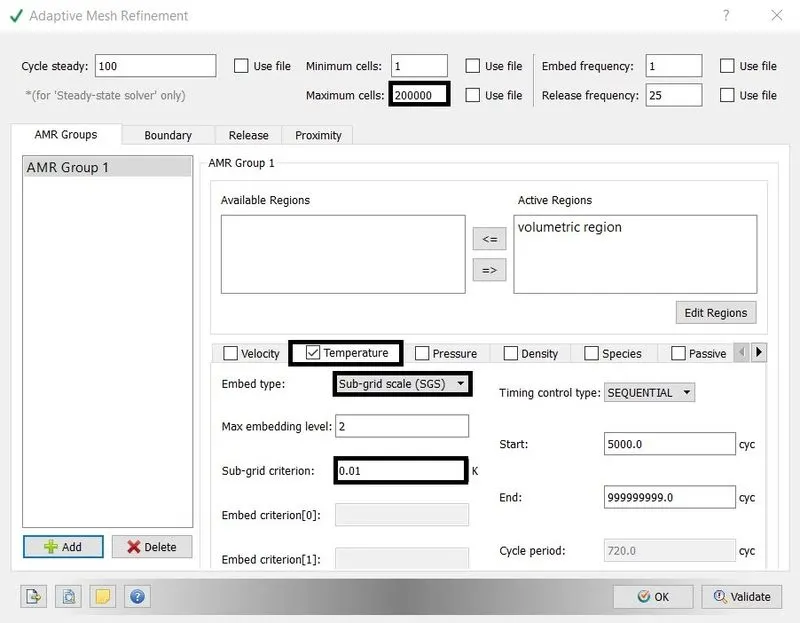
8. Grid Control:-

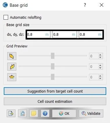
• Base Grid
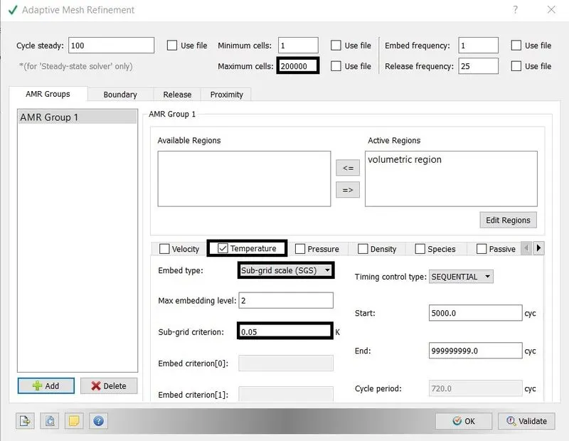
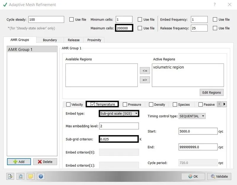
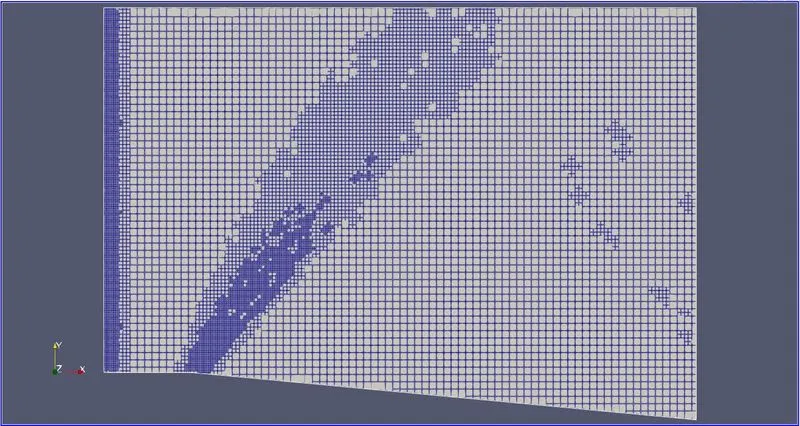
• Adaptive Mesh Refinement (with 0.05K, 0.025K, 0.01K).

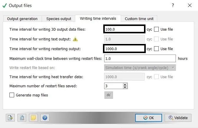
9. Output/Post-Processing:-

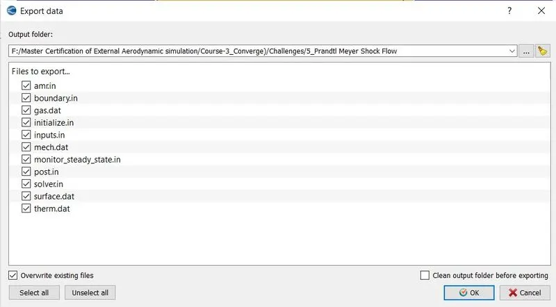
10. Export Data:-

C. Executing the Simulation:-

• The Executable file "mpiexec.exe" and "converge.exe" is pasted in the input files.
• To run the simulation in Cygwin by using the command

mpiexec.exe -n 2 converge.exe restricted </dev/null> logfile &

• After the simulation is complete, the output files can be converted into Ensight format to Post-Process the result in Paraview.

mpiexec.exe -n 2 post_convert_30_msmpi.exe

*******************************************************************************

Case - 1 (Subsonic Flow with SGS temperature of 0.05K)

1. Simulation Time:-

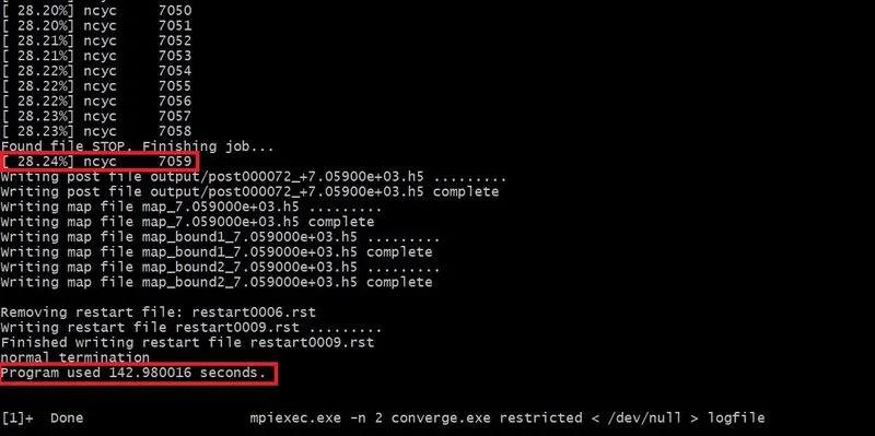
2. Meshing (Surface with edges):-

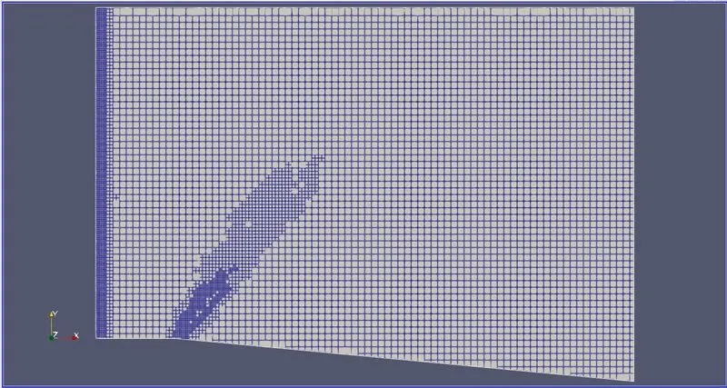
3. Contours:-

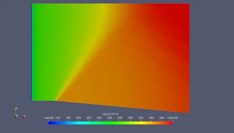
Fig(a). Velocity Contour

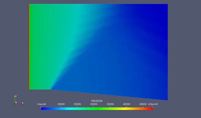
Fig(b). Pressure contour

4. Line Plots for Inlet & Outlet:-

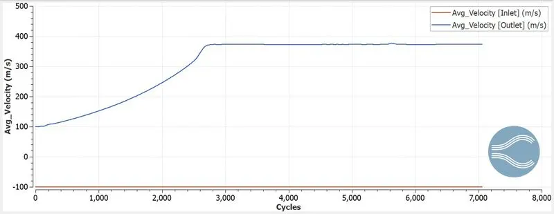
Fig(a). Line plot of Average velocity

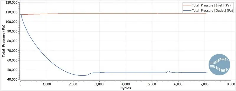
Fig(b). Line plot of Total Pressure

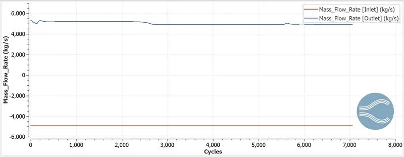
Fig(c). Line plot of Mass Flow Rate

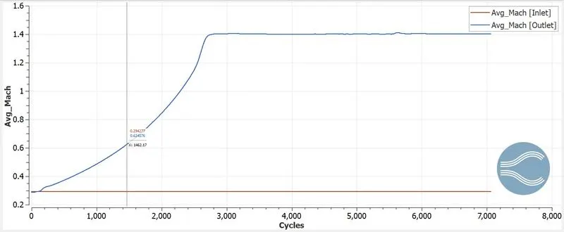
Fig(d). Line plot of Average Mach number

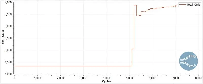
Fig(e). Line plot of Total cells

5. Animations:-

*******************************************************************************

Case - 2 (Subsonic Flow with SGS temperature of 0.025K)

1. Simulation Time:-

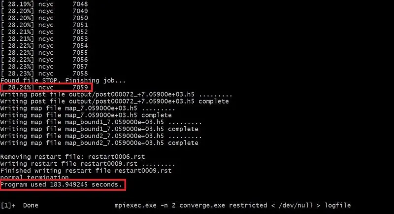
2. Meshing (Surface with edges):-

3. Contours:-

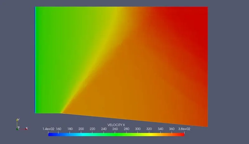
Fig(a). Velocity Contour

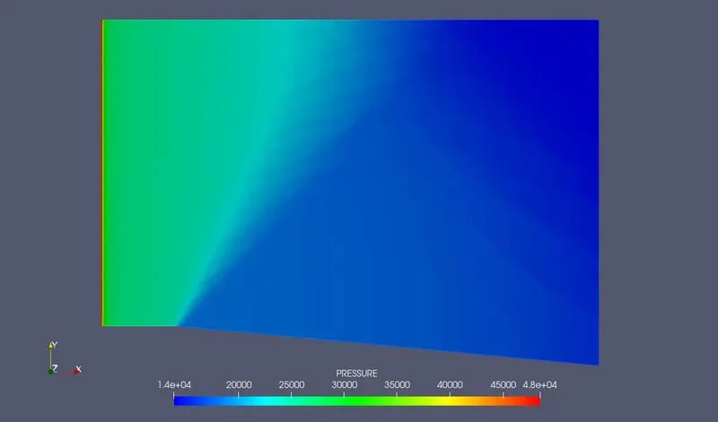
Fig(b). Pressure contour

4. Line Plots:-

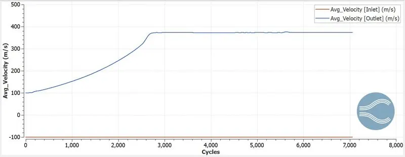
Fig(a). Line plot of Average velocity

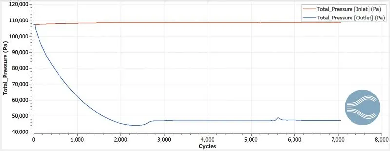
Fig(b). Line plot of Total Pressure

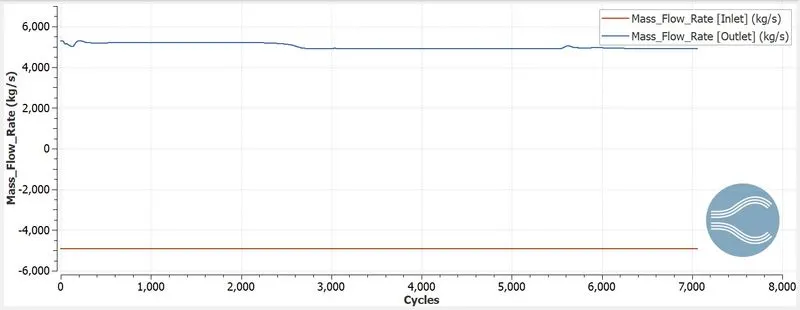
Fig(c). Line plot of Mass Flow Rate

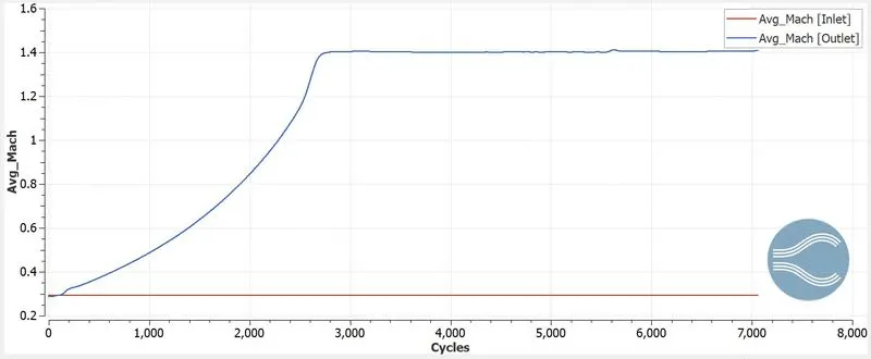
Fig(d). Line plot of Average Mach number

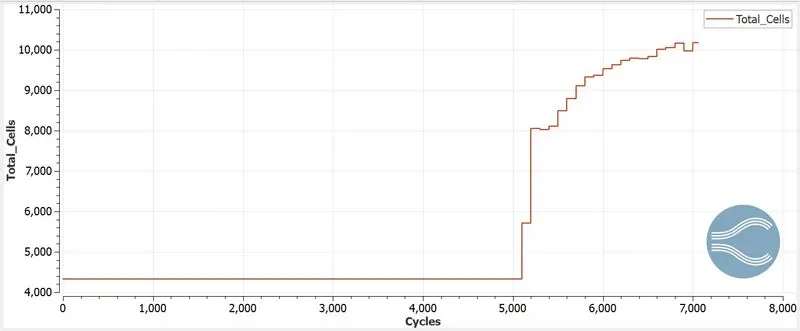
Fig(e). Line plot of Total cells

5. Animations:-

******************************************************************************

Case - 3 (Subsonic Flow with SGS temperature of 0.01K)

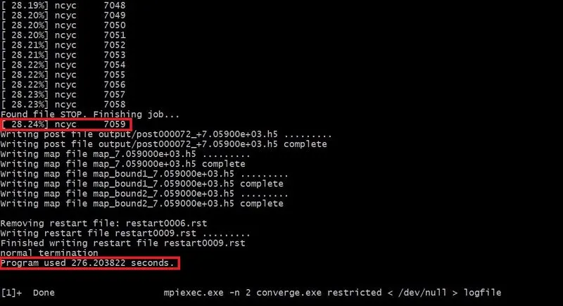
1. Simulation Time:-

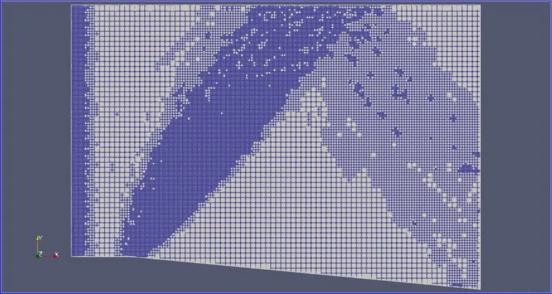
2. Meshing (Surface with edges):-

3. Contours:-

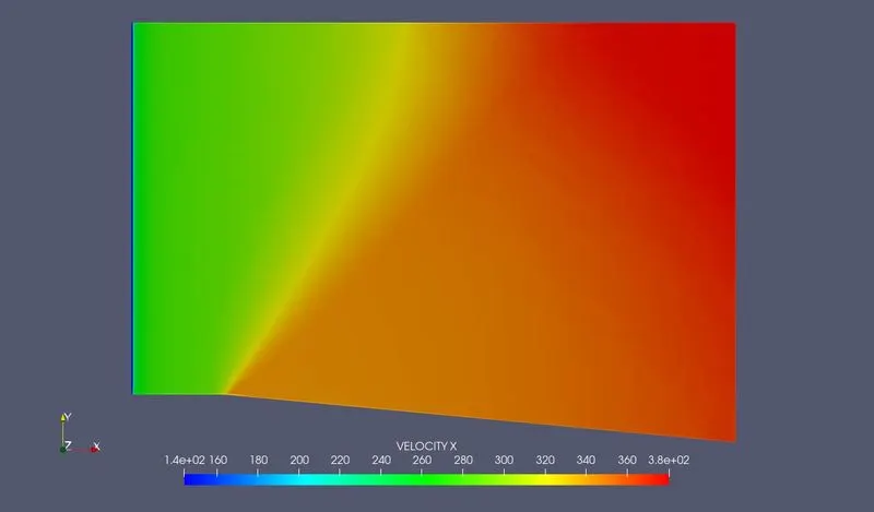
Fig(a). Velocity Contour

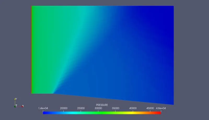
Fig(b). Pressure contour

4. Line Plots:-

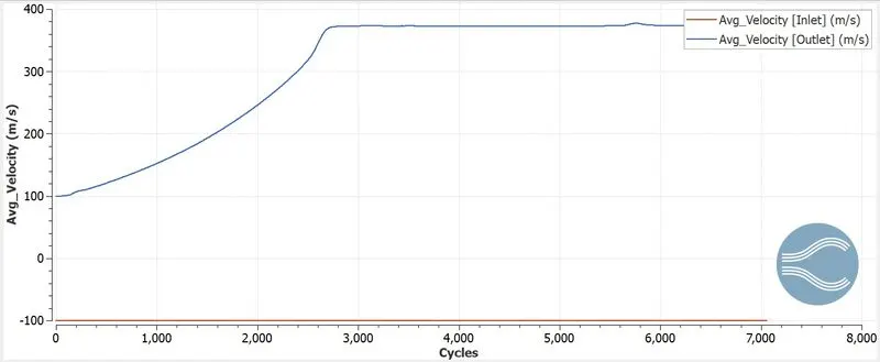
Fig(a). Line plot of Average velocity

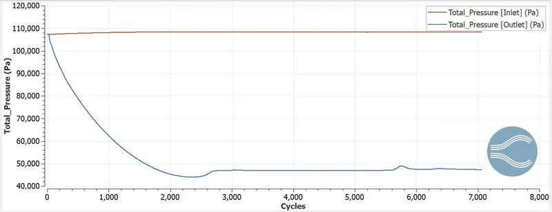
Fig(b). Line plot of Total Pressure

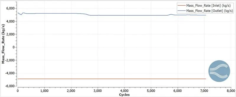
Fig(c). Line plot of Mass Flow Rate

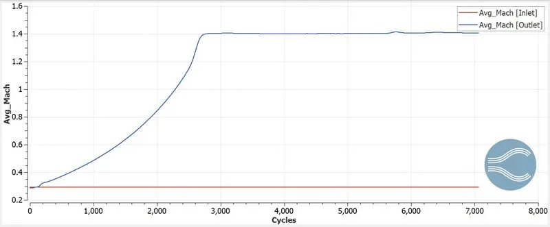
Fig(d). Line plot of Average Mach number

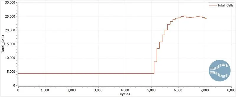
Fig(e). Line plot of Total cells

5. Animations:-

*******************************************************************************

Case - 4 (Supersonic Flow with SGS temperature of 0.05K)

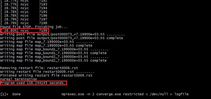
1. Simulation Time:-

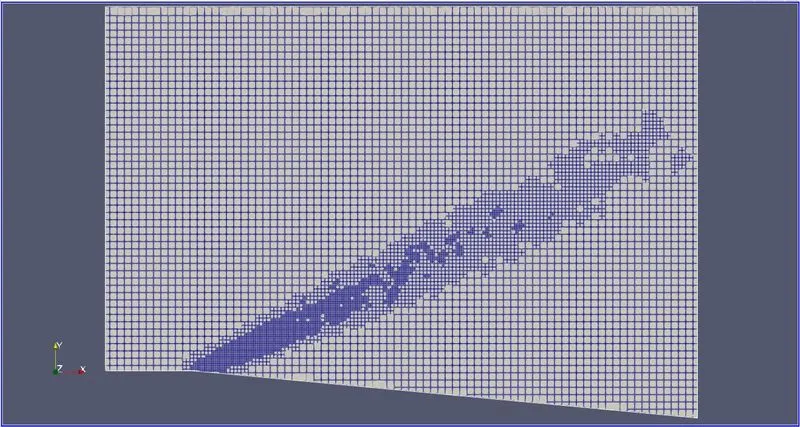
2. Meshing (Surface with edges):-

3. Contours:-

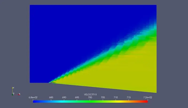
Fig(a). Velocity Contour

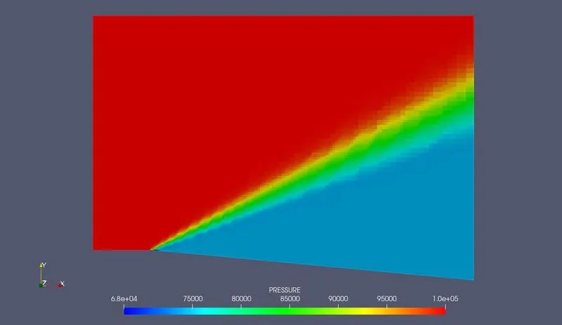
Fig(b). Pressure contour

4. Line Plots:-

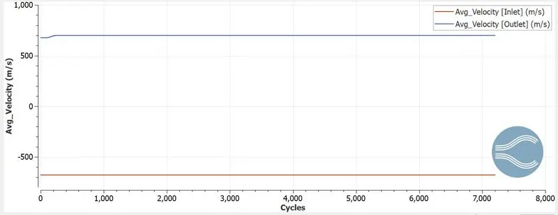
Fig(a). Line plot of Average velocity

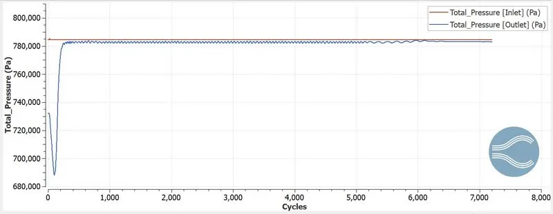
Fig(b). Line plot of Total Pressure

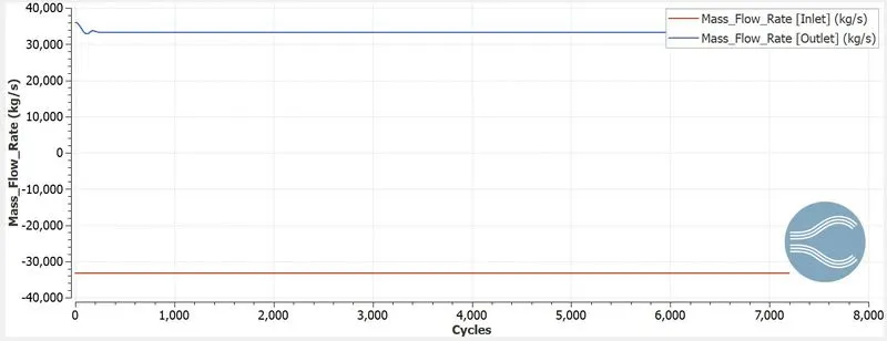
Fig(c). Line plot of Mass Flow Rate

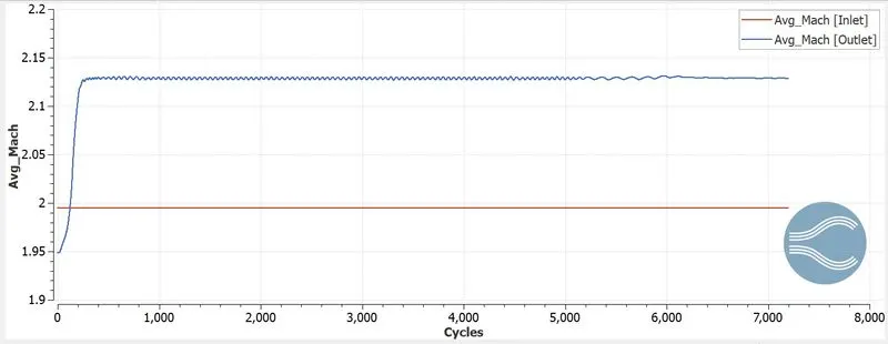
Fig(d). Line plot of Average Mach number

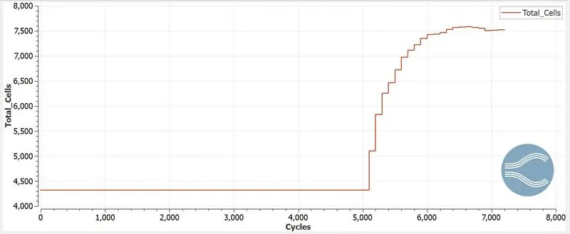
Fig(e). Line plot of Total cells

5. Animations:-

*******************************************************************************

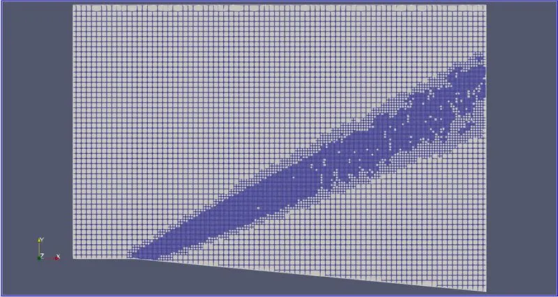
Case - 5 (Supersonic Flow with SGS temperature of 0.025K)

1. Simulation Time:-

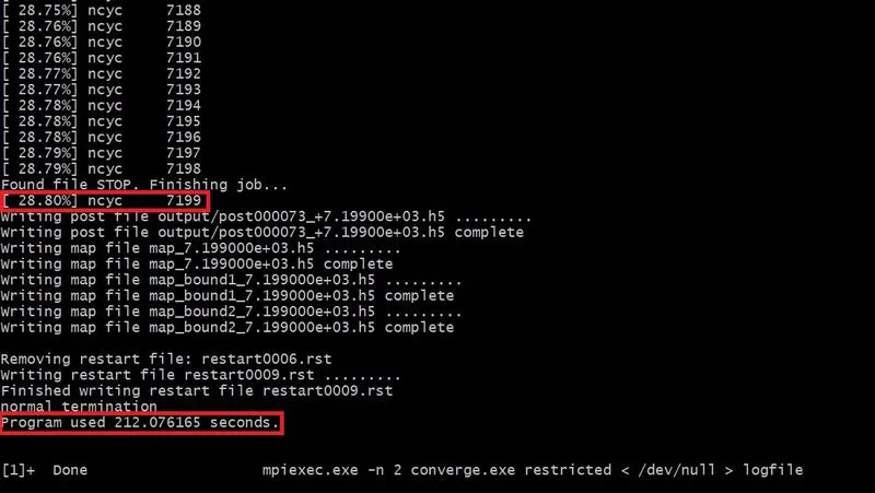
2. Meshing (Surface with edges):-

3. Contours:-

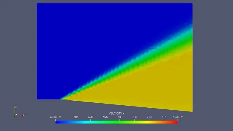
Fig(a). Velocity Contour

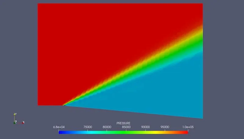
Fig(b). Pressure contour

4. Line Plots:-

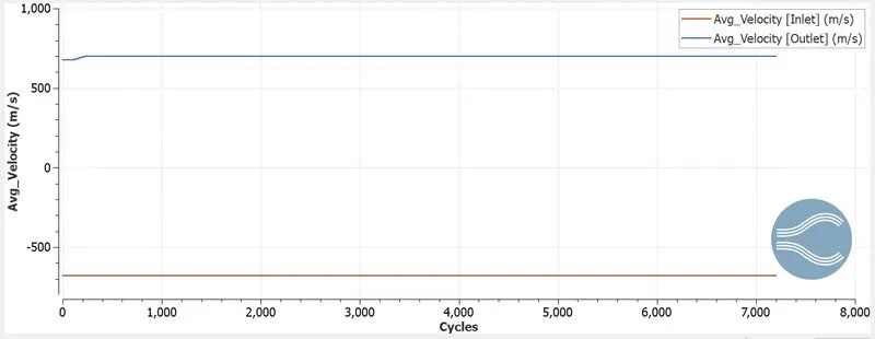
Fig(a). Line plot of Average velocity

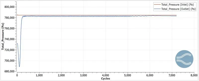
Fig(b). Line plot of Total Pressure

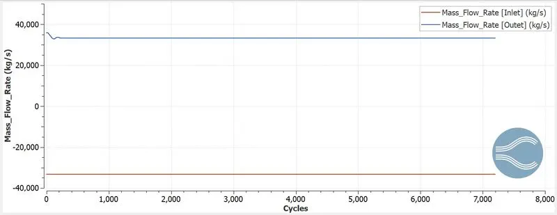
Fig(c). Line plot of Mass Flow Rate

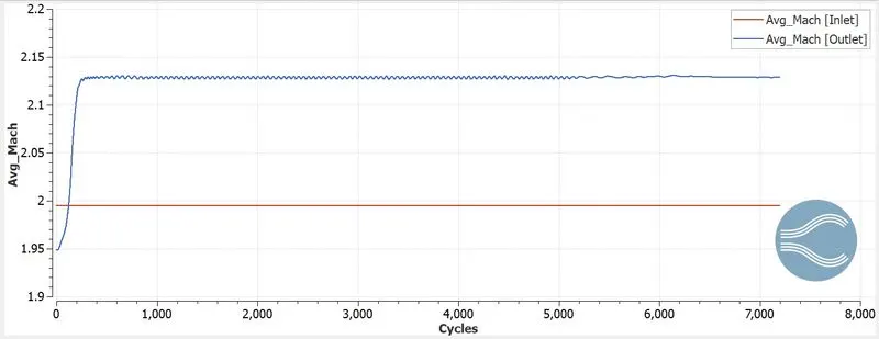
Fig(d). Line plot of Average Mach number

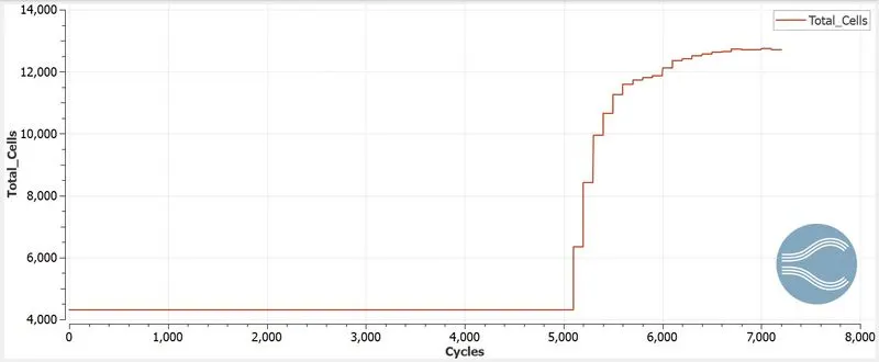
Fig(e). Line plot of Total cells

5. Animations:-

*******************************************************************************

Case - 6 (Supersonic Flow with SGS temperature of 0.01K)

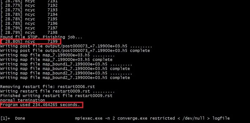
1. Simulation Time:-

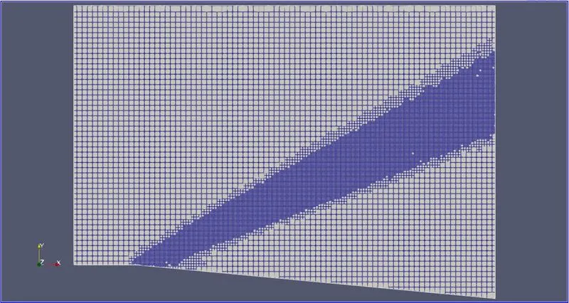
2. Meshing (Surface with edges):-

3. Contours:-

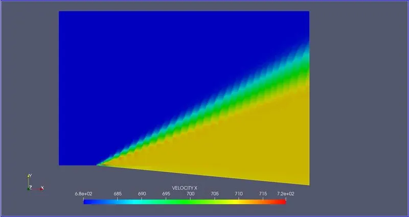
Fig(a). Velocity Contour

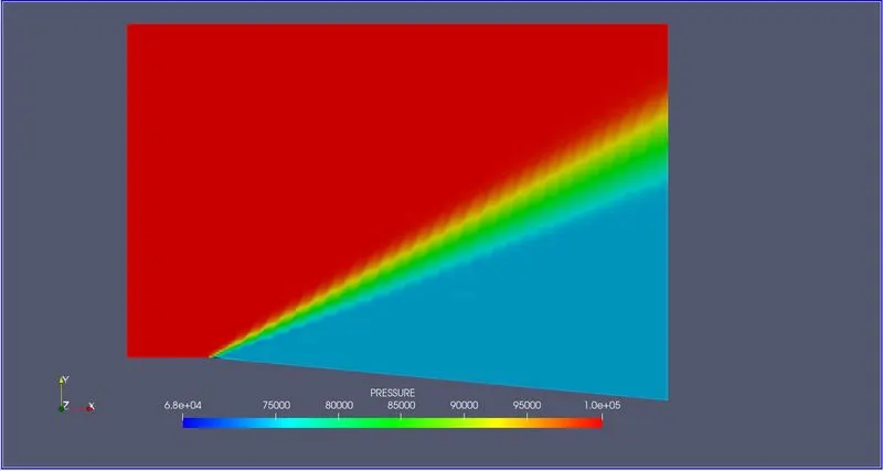
Fig(b). Pressure contour

4. Line Plots:-

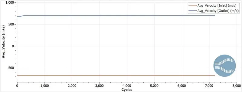
Fig(a). Line plot of Average velocity

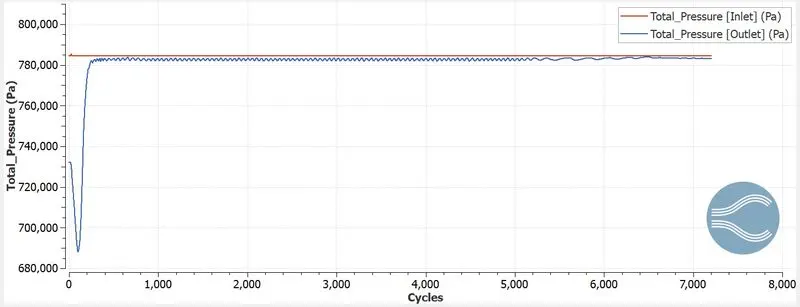
Fig(b). Line plot of Total Pressure

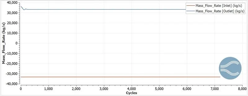
Fig(c). Line plot of Mass Flow Rate

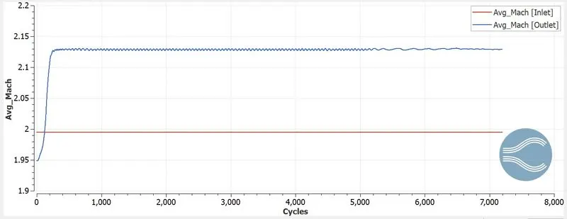
Fig(d). Line plot of Average Mach number

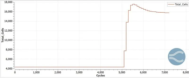
Fig(e). Line plot of Total cells.

5. Animations:-

D. Conclusion:-

Flow Type	Simulation Time (sec)	Total cell	Velocity at Outlet (m/s)	Pressure at Outlet (Pa)	Mach at Outlet	Mass flow Rate (Kg/s)
Subsonic (0.05K)	142.98	6868	373.15	47048.4	1.40	4912.46
Subsonic (0.025K)	183.94	10172	373.9 0	47127.24	1.40	4911.45
Subsonic (0.01K)	276.20	24275	373.94	47305.77	1.40	4929.7
Supersonic (0.05)	158.24	7522	699.89	782925.71	2.1285	33243.93
Supersonic (0.025)	212.076	12714	699.97	783141.25	2.1289	33239.17
Supersonic (0.01)	234.46	15748	700	783222.59	2.1291	33235.88

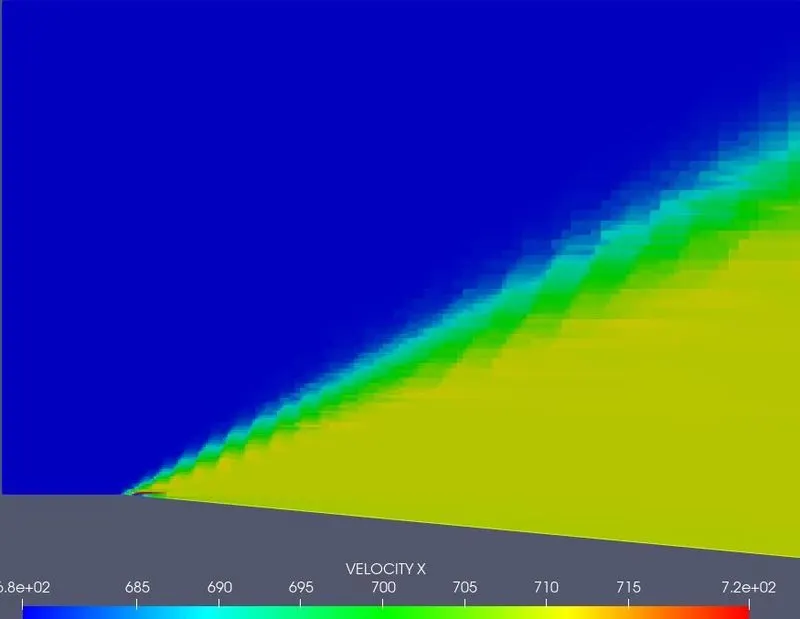
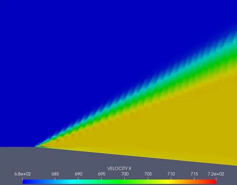
Fig(a). velocity with SGS temperature of 0.05K Fig(b). velocity with SGS temperature of 0.01K

Fig(c). Mesh with SGS temperature of 0.05K Fig(d). Mesh with SGS temperature of 0.01K

• From the Prandtl Meyer simulation, the shock wave has occurred in the supersonic flow.
• The effect of SGS temperature in 0.01K has the shock wave till the end of the outlet but in 0.05K the shock wave is dissolved at a certain range.
• By changing the SGS the pressure, velocity, Mass Flow rate is slightly increased not in much difference.
• The grid capture is finer and accurate while SGS temperature is reduced.
• When the SGS(subgrid scheme) temperature is decreased the total cell count is increased.
• Mach number at the outlet is 2.12.
• The flow accelerates and the Mach number increases, while the static pressure, temperature and density decrease. Since the process is isentropic, the stagnation properties remain constant across the fan.