Prandtl Meyer Shock problem

Introduction

In this study, supersonic flow will be studied using Converge CFD. Before doing so, the following topics will be discussed in brief:

Shock waves

• Neumann boundary conditions

1. Shock waves:

Supersonic flow occurs when the speed of fluid is much greater than the speed of sound in the same medium, with the Mach number M generally being above 1. With an abrubt change in pressure or temperture, the flow adjusts by forming shock waves, with the flow becoming less supersonic.

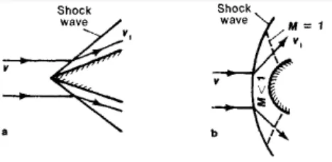
Fig. Supersonic flow (a) wedge (b) blunt body. Click to view source and learn more.

A Prandtl shock expansion fan occurs when supersonic flow turns at a sharp corner, leading to infinite shock waves diverging from this corner.

2. Neumann boundary conditions

The problem with supersonic flow is that there exist no determinable boundary conditions to be applied at the outlets. No information is available at upstream of the shock, and hence zero gradient pressure and velocity boundary conditions are applied at the outlets. This is the Neumann boundary condition.

Aim

• To use adaptive mesh refinement to capture shock wave propogation.
• To study the effect of chnaging the subgrid scale critieria, which basically means a simple study on how changing the adaptive mesh refinement parameters would affect the results of the Prandtl Meyer shock problem.

Setup

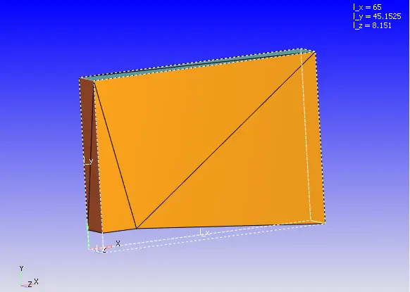
Fig. Geometry

For the setup, compressible steady state solver was chosen. A PISO scheme was adopted for Navier-Stokes equation formulation and solution. The default RNG k-epsilon model was used for turbulent flow. The simulation was run for 25,000 cycles each. In supersonic flow, it is tough to achieve convergence, and hence a high number of iterations (cycles) were run. At the inlet, an inflow boundary condition of 680 m/s was applied, whereas at the outlets, the Neumann zero gradient boundary conditions were applied for pressure and velocity. Top and bottom were set to wall, where as front and back of the gometry were set to 2D to save computational time. The maximum CFL convection limit was set to 0.5 to ensure that the solution does not diverge. Finally, the whole region was initialized with a velocity of 680 m/s, similar to the inlet boundary condition.

Coming to the meshing process, a uniform grid size of 0.8 m was chosen for dx dy and dz. Three cases of subgrid scale criteria dependent on Temperature were chosen, i.e. for example, if the subgrid scale criteria was 0.05, with a change of 0.05 K, the mesh would adaptively refine in those regions. The criteria was chosen as 1, 0.05, and 0.02. In all cases, the mesh refining was made to start only after 5000 cycles.

Results

Case 1: Subgrid criteria - 1

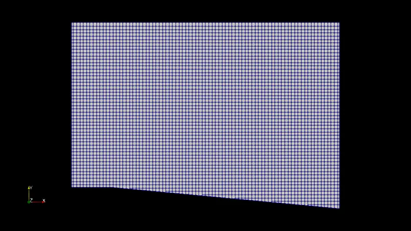
Fig. Final mesh. (Note: no animation is depicted since there is no adaptive mesh refinement for the chosen criteria).

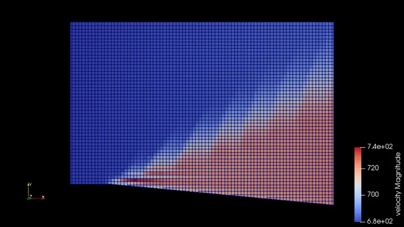
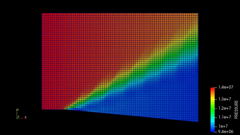
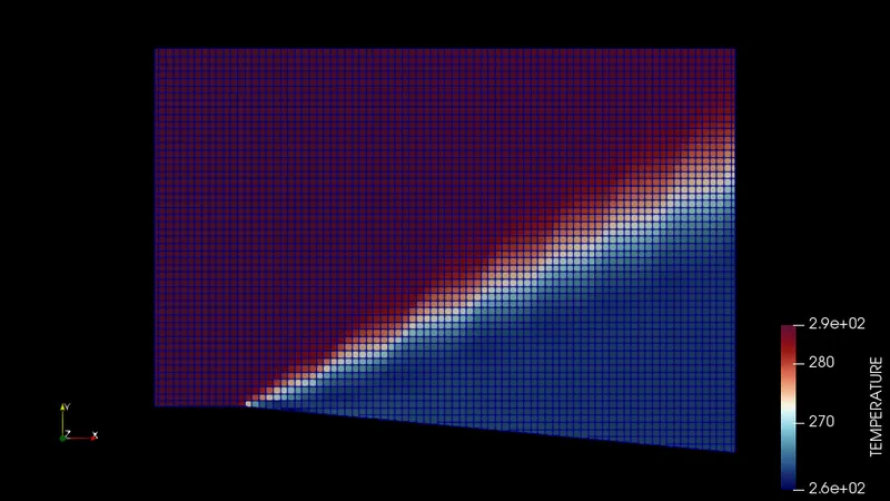
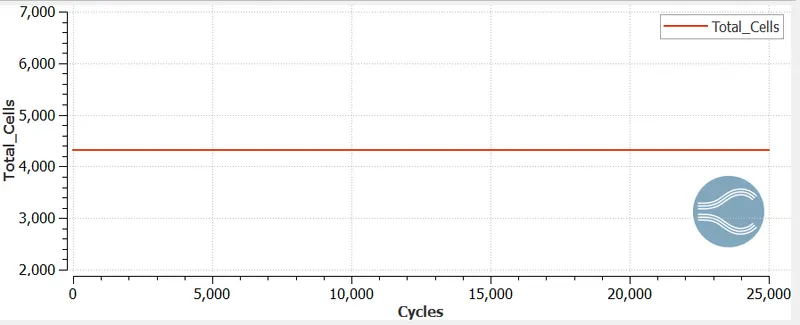
Fig. Velocity, Pressure, Temperature, and Cell count.

Case 2: Subgrid criteria - 0.05

Here, adaptive meshing can be observed for the shock waves, as the solution approaches a steady state. The animation is for velocity.

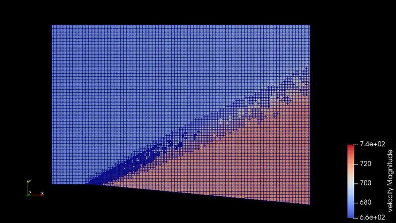
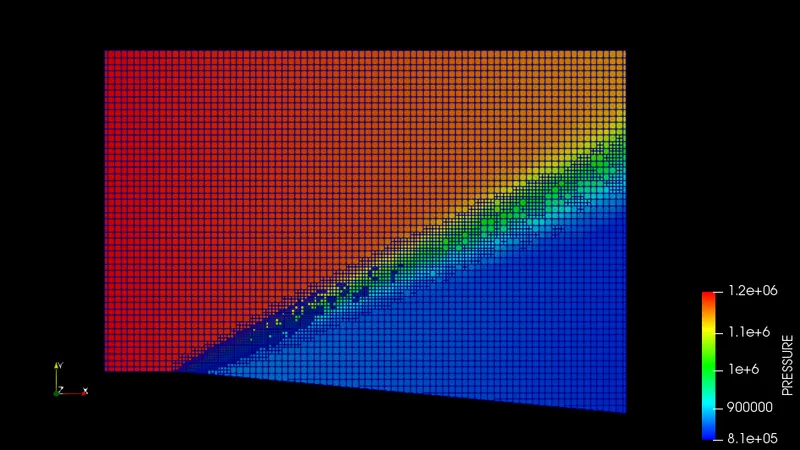
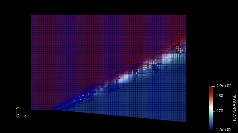
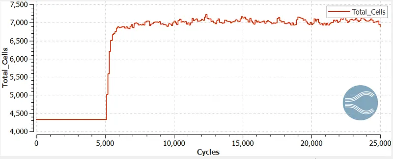
Fig. Velocity, Pressure, Temperature, and Cell count.

Case 3: Subgrid criteria - 0.02

Here, adaptive meshing can be observed for the shock waves, as the solution approaches a steady state. The animation is for pressure.

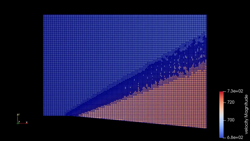
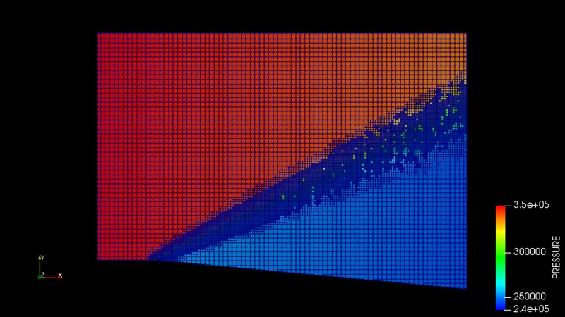
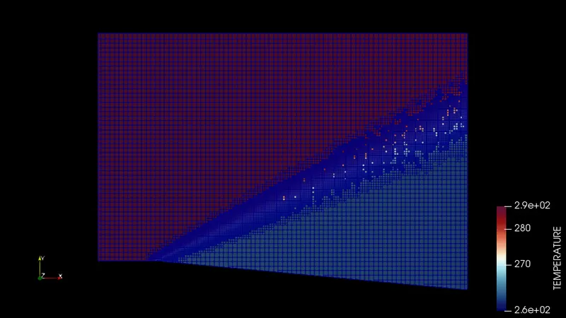
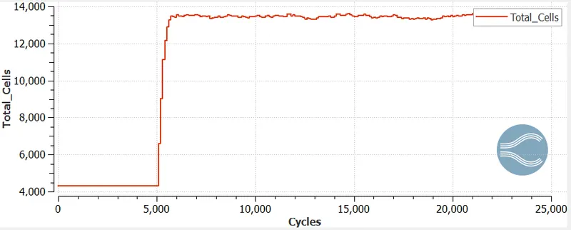
Fig. Velocity, Pressure, Temperature, and Cell count.

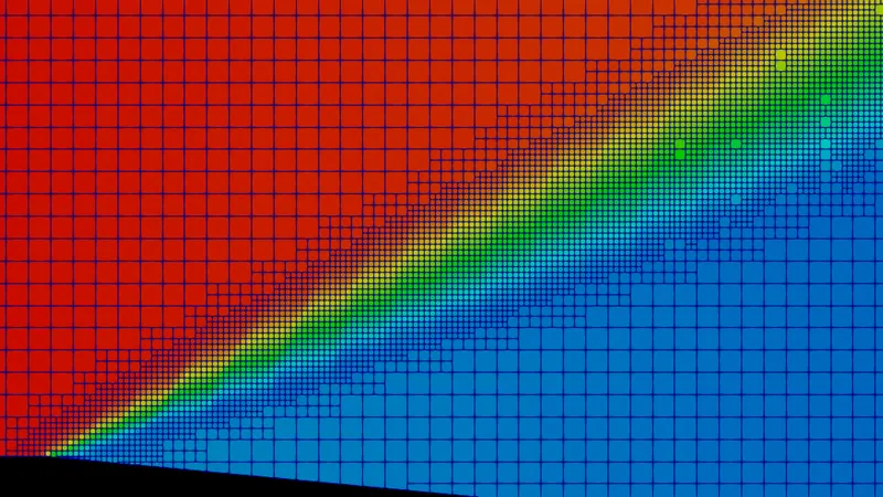
Fig. Close up view of pressure shock waves, with adapative refining.

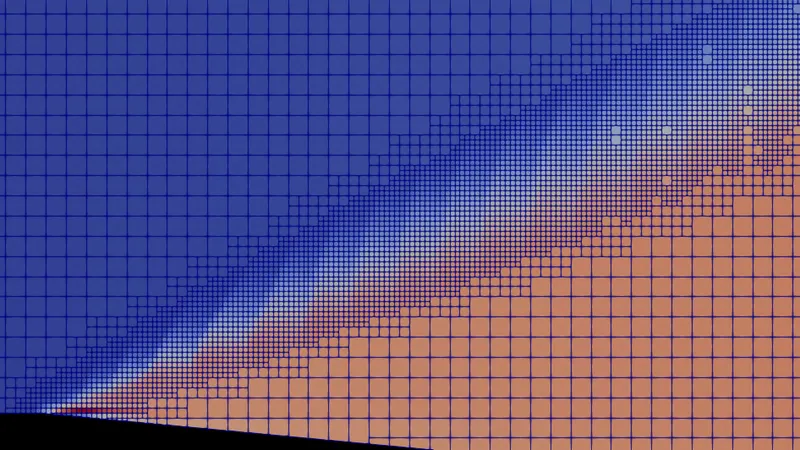
Fig. Close up view of velocity shock waves, with adapative refining.

Conlusion

In this study, a Prandtl Meyer shock problem was simulated using Converge CFD. Adaptive refinement was chosen:

In case 1, no fine cells were used even though adaptive meshing was enabled, meaning the subgrid criteria was not enough to capture the changes in the shock wave.

In cases 2 and 3, an increased cell count was seen, with case three having the lowest sub grid criteria, with fine cells capturing very minute changes in the shock waves.

However, in case 3, the number of cells also increased by a large amount thus increasing computational time.