Week 5: Prandtl Meyer Shock problem

Aim: Simulation of Prandtl Meyer shock flow problem using Converge-CFD and post-process the results.

Objectives:

• literature search on what BC's are typically used for shock flow problems
• What is a shock wave.
• Effect of SGS parameter on shock location.

Introduction:

Shock Flow boundary conditions:

Boundary conditions (BCs) for shock flow problems are essential to accurately capture the physical behavior of flows involving shock waves. These conditions are designed to model interactions between shock waves, boundary layers, and external environments.

Boundary conditions in computational fluid dynamics (CFD) and physics are mathematical constraints applied to define the behavior of flow or field variables at the boundaries of a computational domain. They are categorized based on their physical and mathematical nature:

1. Dirichlet Boundary Conditions:

For shock flow problems, Dirichlet boundary conditions are used to prescribe fixed values for certain variables (e.g., velocity, pressure, temperature, or density) at specific boundaries of the computational domain. These conditions are particularly useful for setting up known flow parameters upstream or downstream of a shock wave, or at solid walls.

2. Neumann boundary conditions

In shock flow problems, Neumann boundary conditions specify the gradient of a variable (e.g., velocity, pressure, or temperature) at the boundary rather than its value. These conditions are particularly useful when the exact values at the boundary are not known, but the flux or derivative is critical to the problem's physics.

In supersonic flows, the flow leaves the domain without upstream influence, so the gradient of variables normal to the boundary is often set to zero: $$\frac{\partial \phi}{\partial n} = 0,$$where ϕ represents velocity components (u, v), pressure (p), or temperature (T).

3. Mixed Boundary conditions

Mixed Boundary Conditions in shock flow problems involve the simultaneous application of different types of boundary conditions (e.g., Dirichlet, Neumann, and Robin) on the same domain boundary or across different boundaries. These conditions are tailored to the physical behavior of the flow and the characteristics of the boundary.

4. Robin Boundary conditions:

Robin Boundary Conditions are a combination of Dirichlet and Neumann boundary conditions and are often used in problems involving convection, diffusion, and heat transfer. In the context of shock flow problems, Robin conditions are used to model more complex interactions at boundaries, such as heat flux with specified surface temperatures or conditions involving convective outflows.

What is a shock wave ?

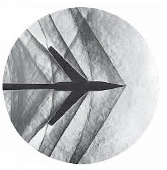
A shock wave is a type of propagating disturbance in a medium (such as air, water, or a solid) characterized by a sudden and dramatic change in properties such as pressure, temperature, and density. It is caused when an object moves through the medium at a speed faster than the local speed of sound (i.e., supersonic speeds), or when a rapid release of energy occurs, as in an explosion.

Shock waves are formed when a pressure front moves at supersonic speeds and pushes on the surrounding air. At the region where this occurs, sound waves travelling against the flow reach a point where they cannot travel any further upstream and the pressure progressively builds in that region; a high-pressure shock wave rapidly forms.

Equations Governing Shock waves

Shock waves obey the Rankine-Hugoniot relations, derived from conservation laws:

1. Conservation of Mass:
   ρ_1​u₁​=ρ₂​u₂​
2. Conservation of Momentum:
   p_1​+ρ_1​u₁²​=p₂​+ρ₂​u₂²​
3. Conservation of Energy:
   h_1​+u₁²/2^​​=h₂​+u₂2/2 ​where:

• ρ: Density
• u = velocity
• p= pressure
• h: Specific enthalpy

Shock waves are associated with an increase in entropy, making the process inherently irreversible. This results in energy dissipation, typically as heat.

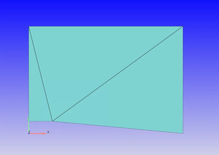
Geometry:

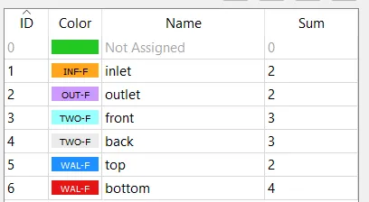
Boundary flagging:

Flag the geometry boundaries, respectively.

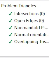
Diagnosis:

check the diagnosis tool to find out the geometry errors

Case Setup:

application type: Time-based

Materials:

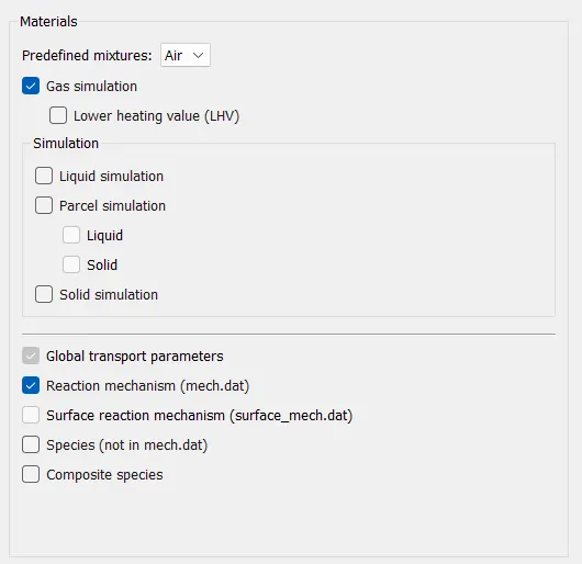
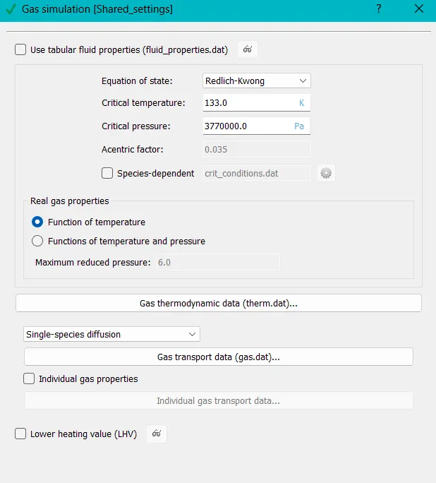
Gas simulation:

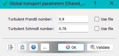
Global transport parameters:

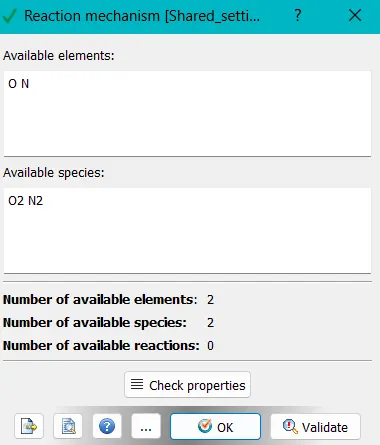
Reaction mechanism:

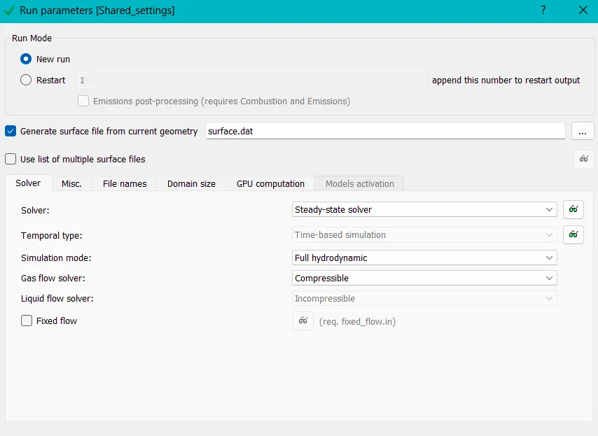
Run parameters:

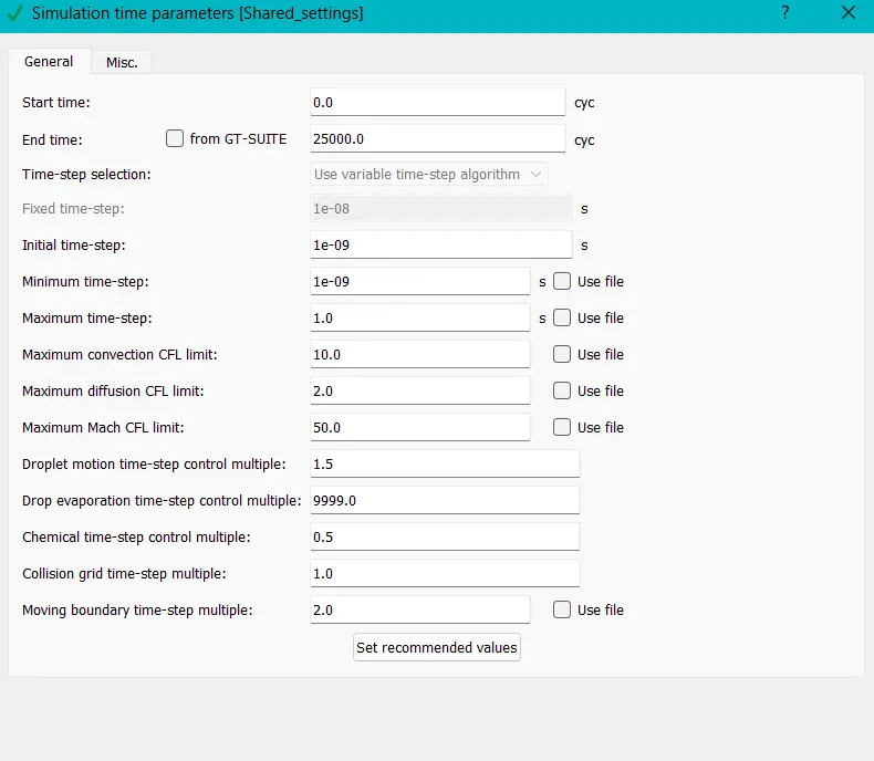
Simulation Time parameters:

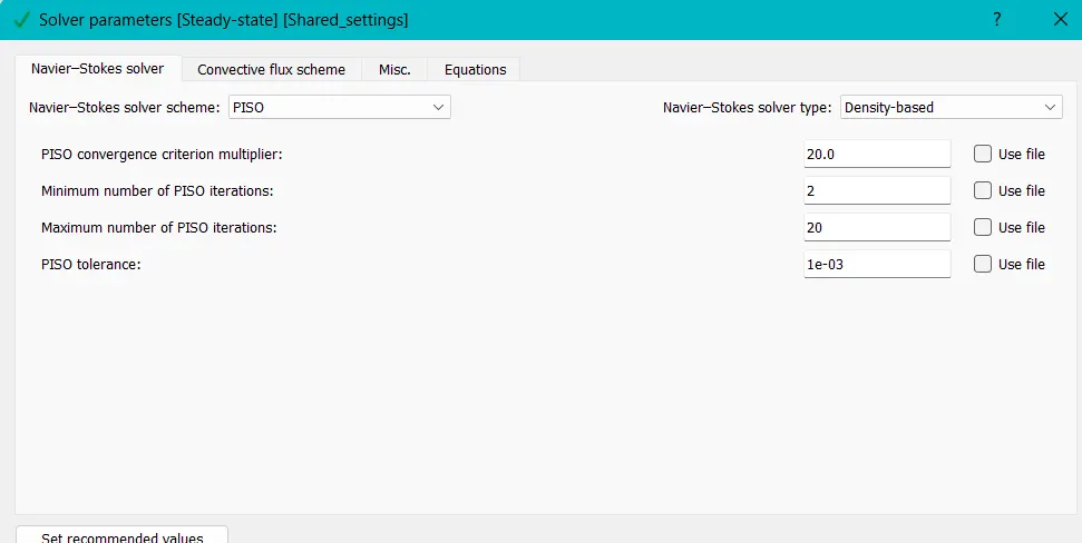
Solver parameters:

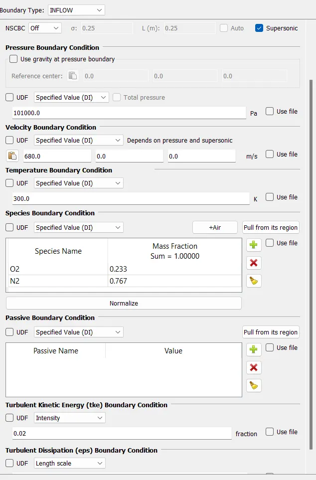
Boundary Conditions:

Inlet:

Outlet:

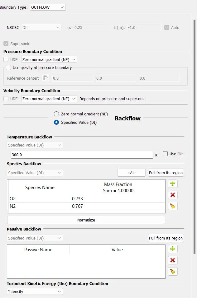
Front and Back :

boundary Type --> Two_D

Top and Bottom:

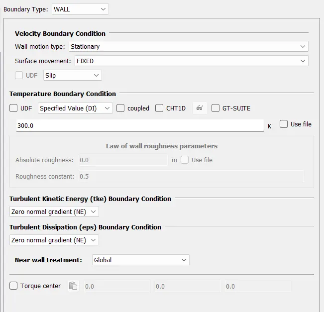
Regions and Initiaization:

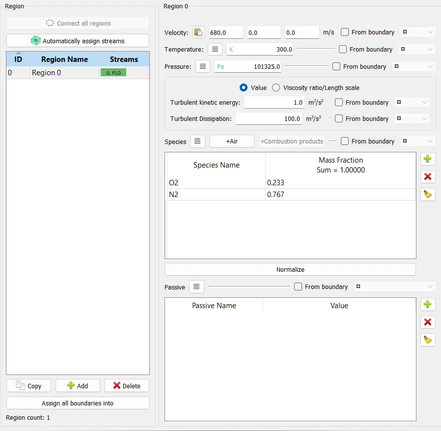
Turbulence model: RNG K-epsilon.

Base grid:

dx=1.3m; dy=1.3m; dz=1.3m

Adaptive mesh refinement:

Case_1: SGS = 0.01m

Case_2: SGS = 0.005m

max cells = 2000000

Output files:

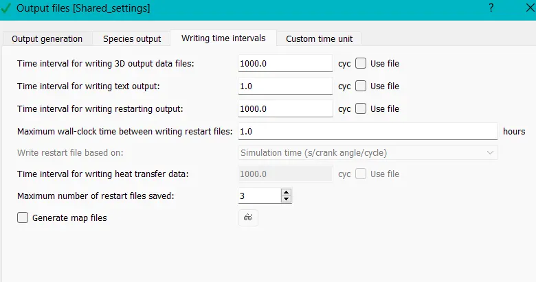
Running the Simulation:

• Open cygwin and navigate into the case directory where we exported the case setup input files.
• Run the following command
  $ mpiexec -n 4 converge --license explore
  
• This commands checks the license and converges the test case and generates output files.
• The to post process the results in Paraview, the output files are converted into group file format that supports in paraview.

Post-Processing:

case_1:

SGS = 0.01

Mesh:

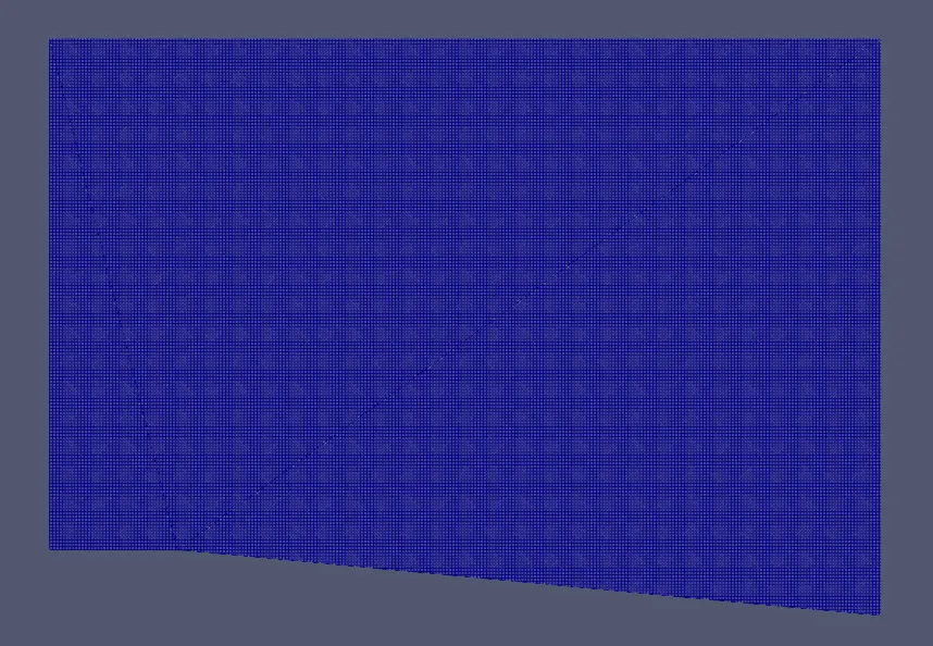
tempersture animation:

https://youtu.be/29v9EFaEUcM

Pressure animation:

https://youtu.be/zH3l_cSJfdY

Velocity animation:

https://youtu.be/aGUvnXTcsi8

Case_2:

SGS =0.05

Mesh:

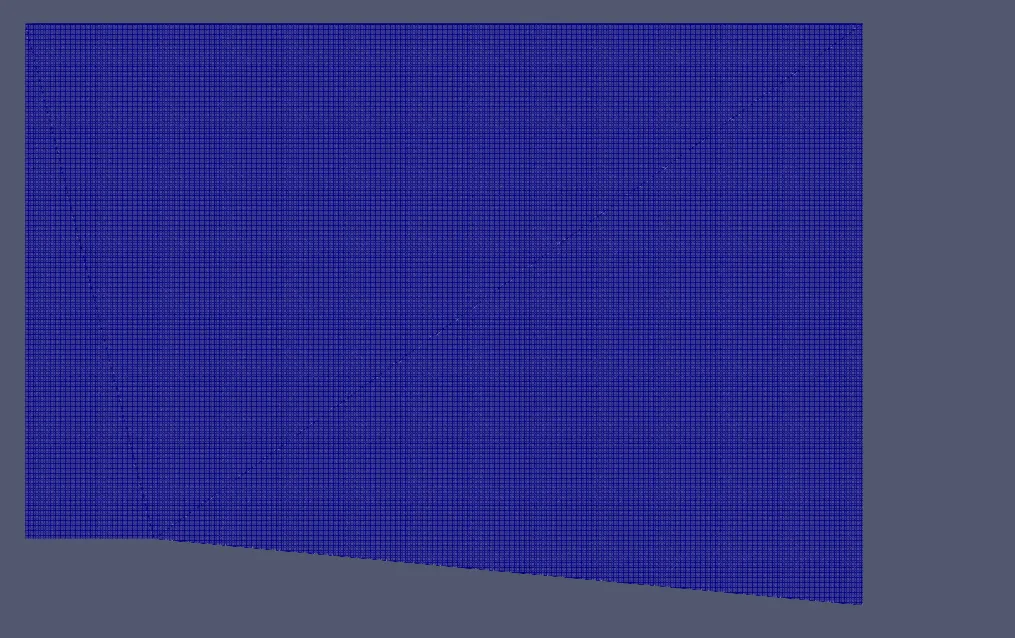
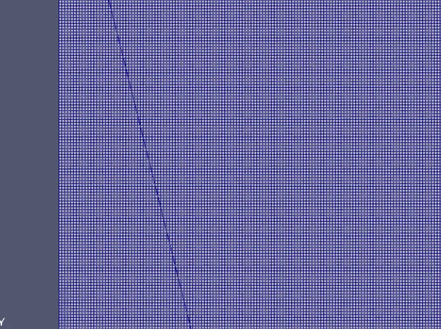
Temperature animation:

https://youtu.be/rT7_DTu6iqg

Pressure animation:

https://youtu.be/PPtQZFncw4Q

Velocity animation:

https://youtu.be/4ZaDCMm9EZE

Case_3:

SGS =0.1

Mesh:

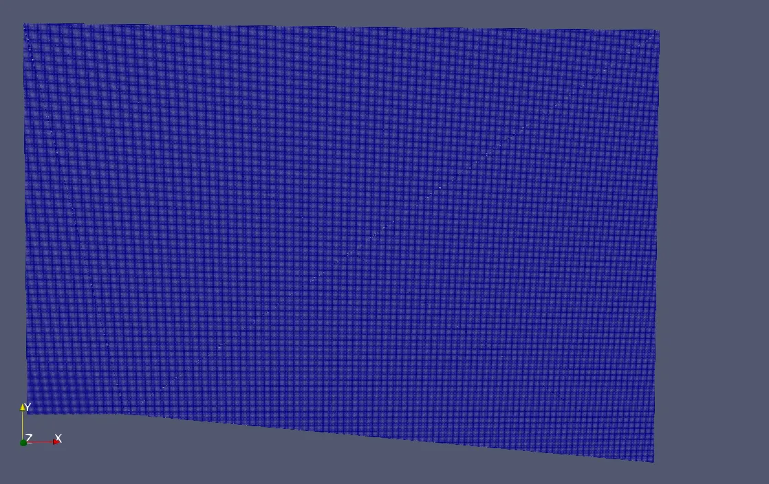
temperature animation:

https://youtu.be/SJd2C9zabkU

Pressure animation:

https://youtu.be/jnE6pT7Ikxc

Velocity animation:

https://youtu.be/ohH-KSs7U6E

Comparison plots:

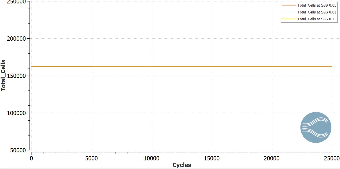
Total cells vs cycle:

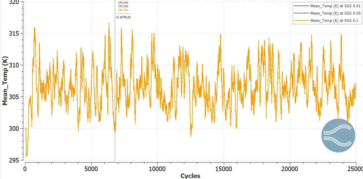
Average Temperature vs cycle:

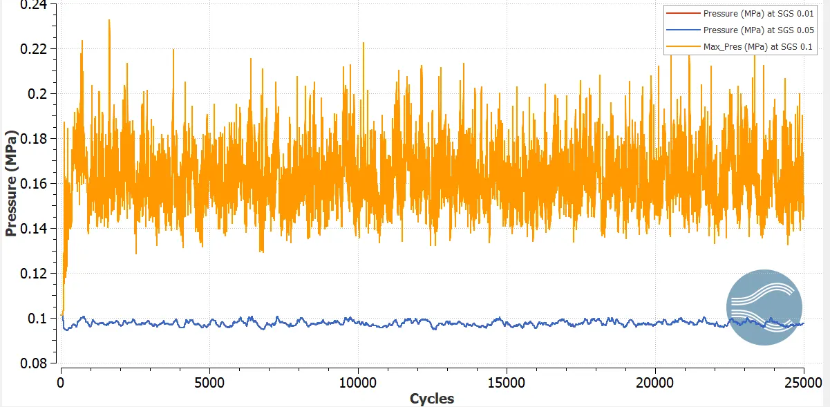
Pressure vs Cycle:

Conclusion:

Here, we performed the Simulation of Prandtl Meyer shock flow problem using Converge-CFD and post-process the animation results and also compared the results in three different SGS case values. The main observation in this simulation is the mesh getting finer, when the SGS value decreases, that minimizes the error rate.