Week 5: Prandtl Meyer Shock problem
Your Answers
Prandtl Meyer Shock problem
1. Shock flow boundary conditions
Do a literature search on what BC's are typically used for shock flow problems
2. What is a shock wave?
In your own words, describe the physics behind shock waves
3. Effect of SGS parameter on shock location
In the Prandtl Meyer shock problem, look at the effect of SGS temperature value on cell count and the shock location
Answer
Shock Flow Boundary Conditions
Boundary conditions (b.c.) are constraints necessary for the solution of a boundary value problem. A boundary value problem is a differential equation (or system of differential equations) to be solved in a domain on whose boundary a set of conditions is known. It is opposed to the “initial value problem”, in which only the conditions on one extreme of the interval are known. Boundary value problems are extremely important as they model a vast amount of phenomena and applications, from solid mechanics to heat transfer, and from fluid mechanics to acoustic diffusion.
Different Types of Boundary Conditions for a Shock Flow
1. Dirichlet BC
The Dirichlet boundary condition is a type of boundary condition named after Peter Gustav Lejeune Dirichlet (1805–1859).
Dirichlet boundary conditions also referred to as first-type boundary conditions, prescribe the numerical value that the variable at the domain boundary should assume when solving the governing ordinary differential equation (ODE) or partial differential equation (PDE). In fluid dynamics, it is usually the pressure or velocity values that are imposed on the boundary of the domain. For instance, when solving fluid dynamics problems for a viscous fluid with no-slip and no-penetration conditions, according to the Dirichlet boundary condition, the component of velocity should be zero at the boundary.
When solving the ordinary differential equation, y”+y=0, the Dirichlet boundary condition for the interval (a,b) can be expressed as y(a) =α and y(b)=β, where α and β are the fixed given numbers.
2. Neumann BC
In mathematics, the Neumann (or second-type) boundary condition is a type of boundary condition named after a German mathematician Carl Neumann (1832–1925). When imposed on an ordinary or a partial differential equation, it specifies the values that a solution needs to take along the domain’s boundary.In heat transfer problems, the Neumann condition corresponds to a given rate of change of temperature. In other words, this condition assumes that the heat flux at the material’s surface is known. The heat flux in the positive x-direction anywhere in the medium, including the boundaries, can be expressed by Fourier's law of Heat conduction.
3. Robin BC
4. Mixed BC
5. Cauchy BC
Shock Wave
In Physics, a shock wave is also known as shock waves. It is a strong pressure wave in an elastic medium such as air, water, or any solid material ejected from explosions or lightning, or other phenomena that create variations in pressure.It is a type of disturbance that propagates at a speed greater than the speed of sound in the medium. As a rule, like ordinary waves, shock waves carry energy and can propagate through a medium. Above all, we characterize a shock wave by a sudden, nearly discontinuous, change in pressure, temperature, and density of the medium.
When an aeroplane travels at a speed less than that of sound, in the first place, the air stays ahead of it. In the meantime, the air begins to flow out of the way, before the plane approaches it. The pressure waves that aeroplane creates past the air, eventually end up being smooth and gradual.However, when an aeroplane reaches the speed of sound and catches up to its own pressure waves, the air ahead of it receives no signal of the plane’s approach. The aeroplane flows through the air, creating a strong pressure wave known as a shock wave. In this case, when air flows through the shock wave, its pressure, density, and temperature increase sharply and quickly.
Prandtl-Meyer Expansion Fan
A supersonic expansion fan, technically known as Prandtl–Meyer expansion fan, a two-dimensional simple wave, is a centered expansion process that occurs when a supersonic flow turns around a convex corner. The fan consists of an infinite number of Mach Waves, diverging from a sharp corner. When a flow turns around a smooth and circular corner, these waves can be extended backwards to meet at a point.
Each wave in the expansion fan turns the flow gradually (in small steps). It is physically impossible for the flow to turn through a single "shock" wave because this would violate the second law of thermodynamics.
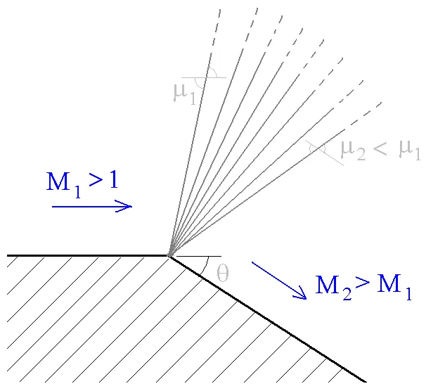
Across the expansion fan, the flow accelerates (velocity increases) and the Mach Number increases, while the static pressure, temperature and density decrease. Since the process is isentropic , the stagnation properties (e.g. the total pressure and total temperature) remain constant across the fan.
The theory was described by Thedor-meyer on his thesis dissertation in 1908, along with his advisor Pradtl, who had already discussed the problem a year before.
Effect of SGS parameter on shock location
In this problem, we start by running the Converge CFD software by building up a case setup of prandyl-meyer expansion fan geometry that represents the parameters to run the data. No where we already have a.STL file so we download it grab the file and drag it to the converge or you can do with the conventional method by opening new projects in the new section.
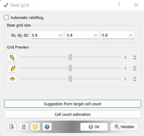
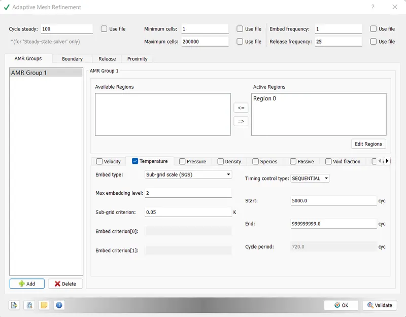
In the given below geometry, the profile was of really high scaling, to reduce the number of grid points and meshing to be smooth and doable therefore, we have reduced to 0.001 scale ratio. That is how we perform a Sub-Grid scaling (SGS).
Case Setup in Converge
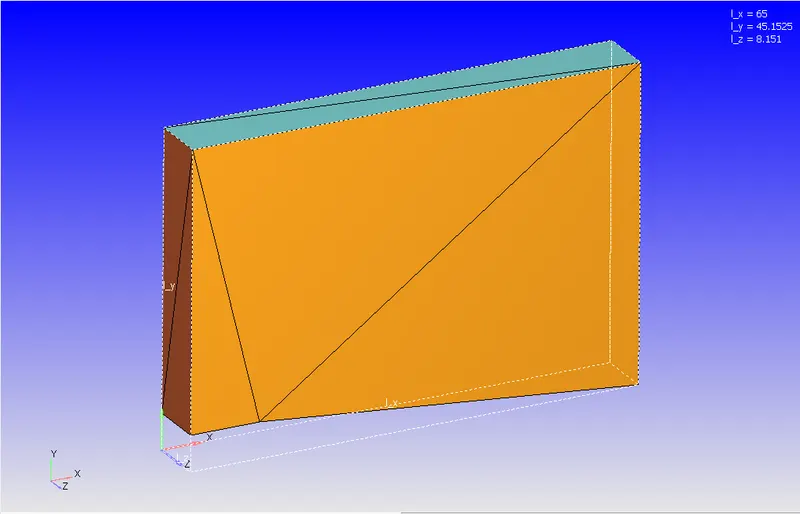
The Geometry. This is a 3D geometry of a divergent nozzle.
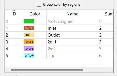
Boundary Assigning
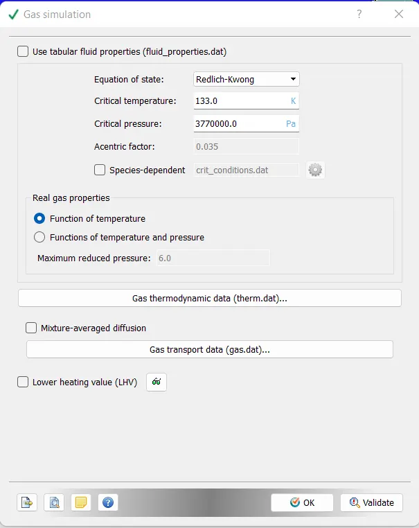
Gas simulation, make it as default.
 ''
''
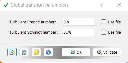
Global Transport Parameters, default settings
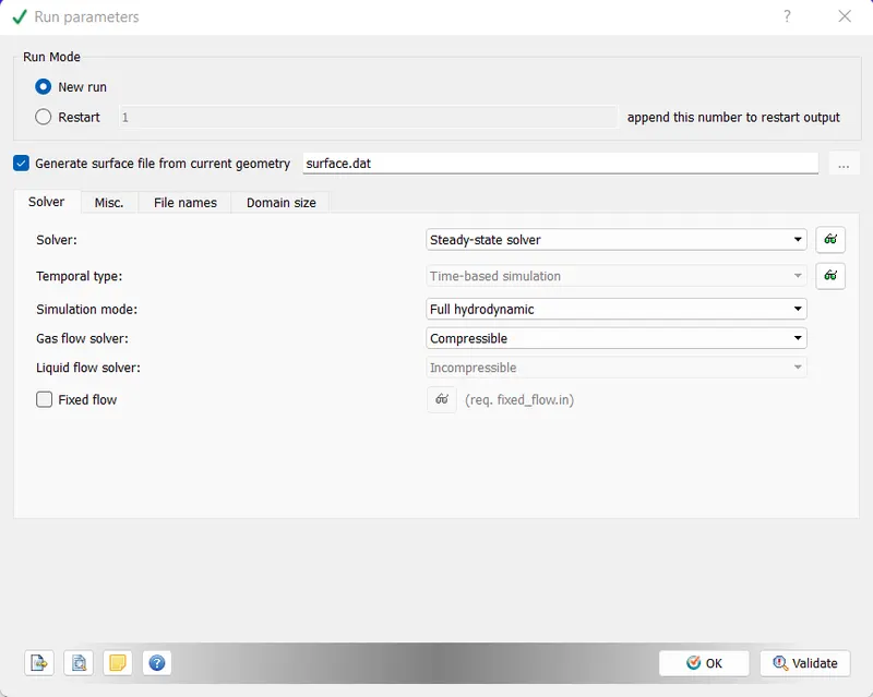
Run Parameters , Solver = Steady-State Solver
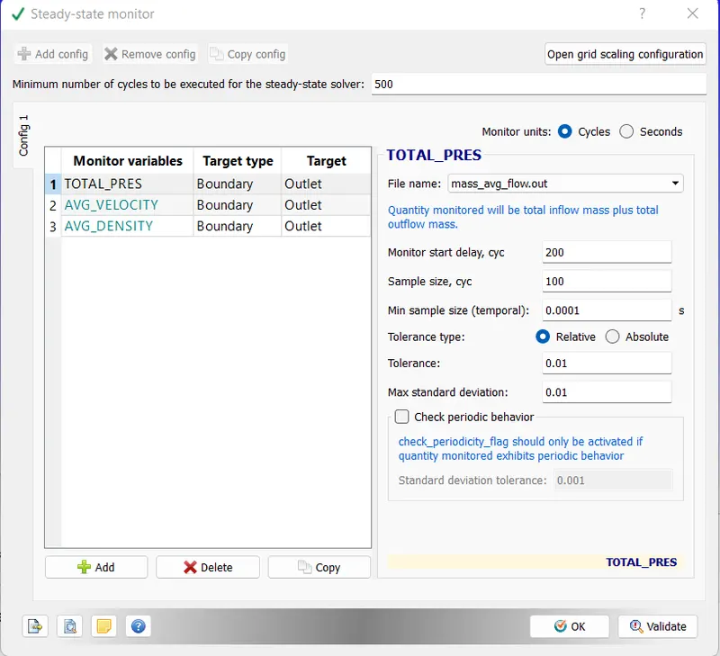
Steady State Monitor setting as this
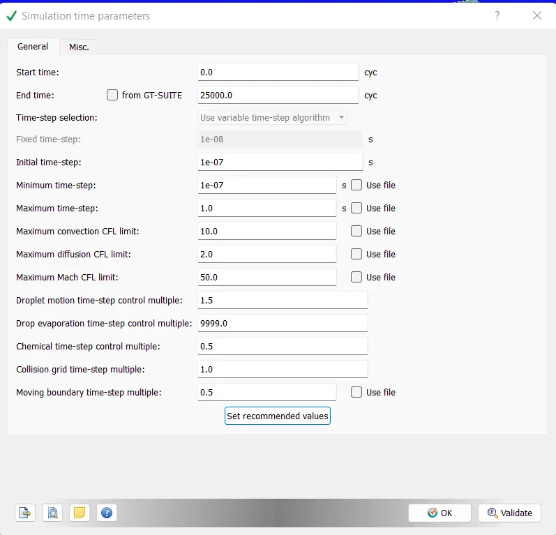
Simulation Time Parametrs
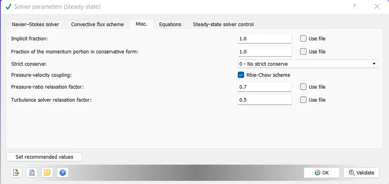
Solver Parameter
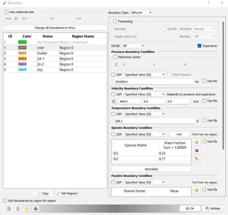
Boundary Condition, Inlet
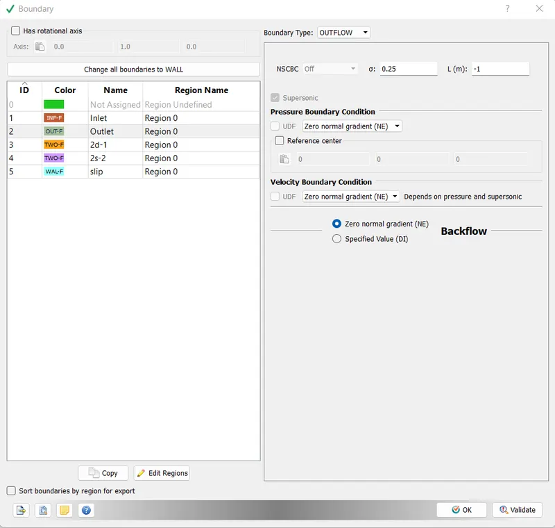
Boundary - Outlet
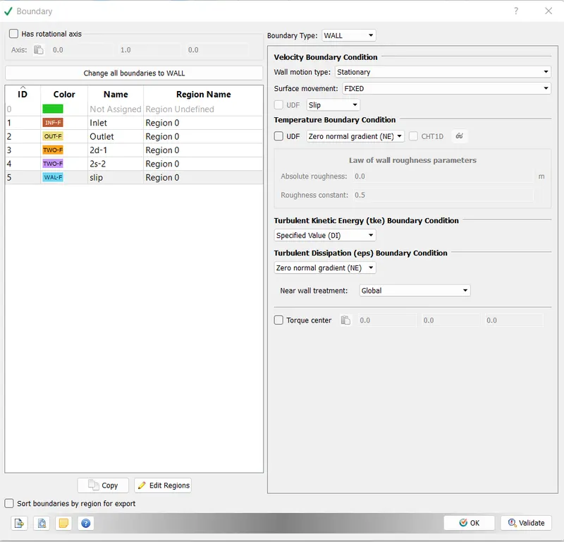
Boundary, Slip
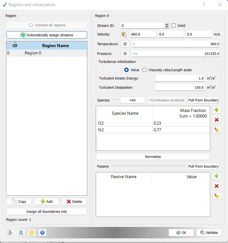
Regions and Initialization
Base Grid Size
Adaptive Mesh refinement
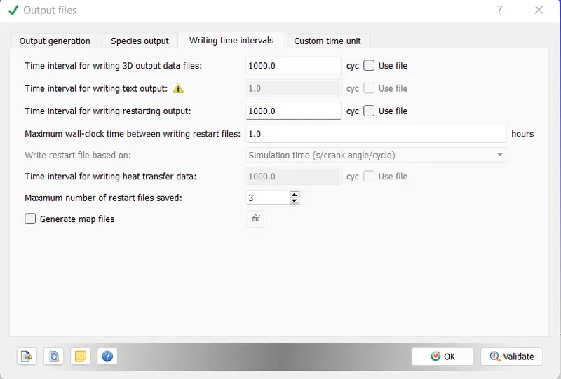
Output Files
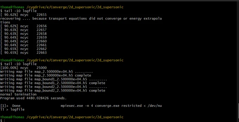
Now, we export the files and start running the simulation on Cygwin.
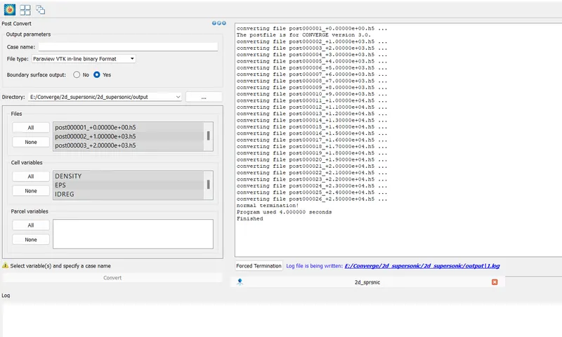
Now, we convert the binary files to paraview readable format using converge
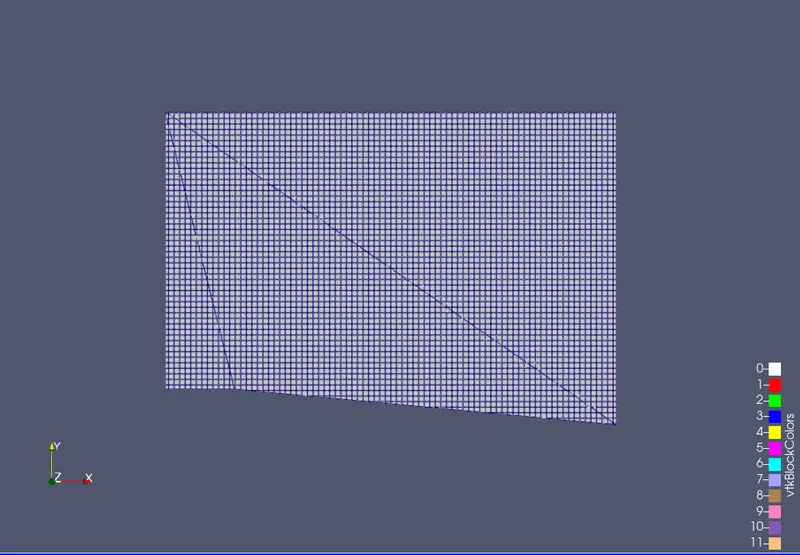
ParaView
The Mesh diagram
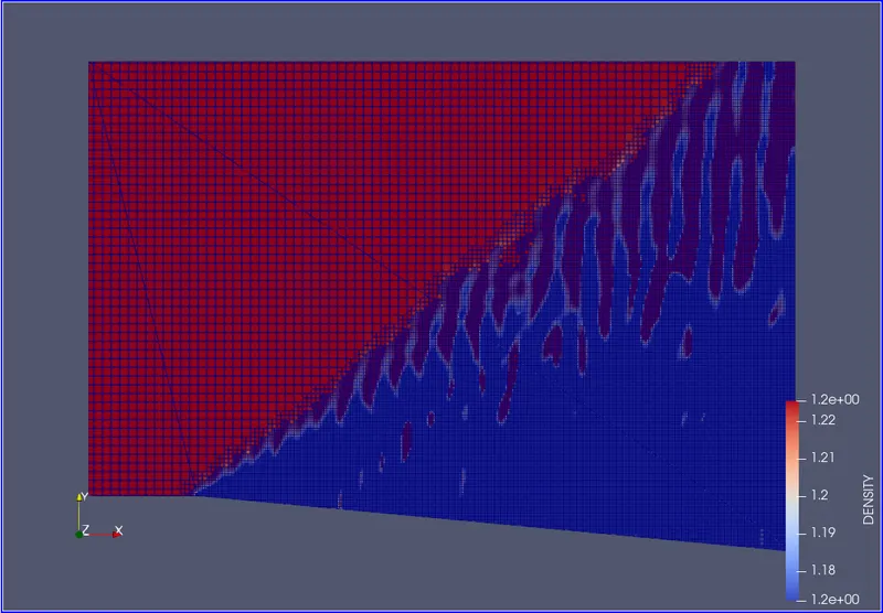
Results
The density contour at last step
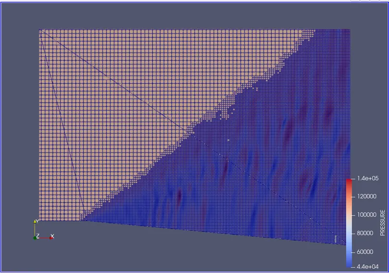
The pressure contour at last step
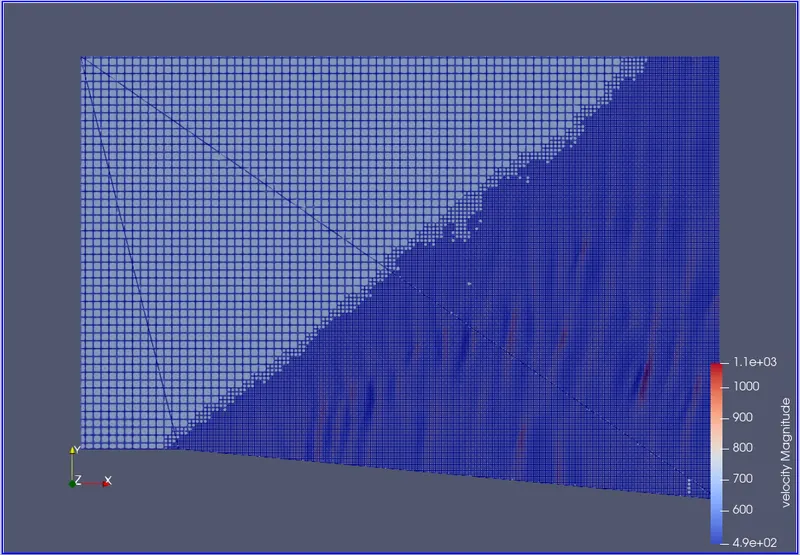
Velocity contour at the last step
Youtube Uploaded Videos
Density
Pressure
Velocity
Thank You