Week 5: Prandtl Meyer Shock problem
Aim: Simulate the prandtl meyer shock flow in converge CFD.
Objective
- To Do a literature search on what BC's are typically used for shock flow problems.
- What is a shock wave?
- To describe the physics behind shock wave.
- Effects of SGS parameter on shock location (Sub-grid-scaling).
Shock flow boundary conditions
Boundry conditions are constraints necessary for the solution of a boundary value problem. A boundary value problem is a differential equation (or system of differential equation) to be solved in a domain on whose boundary a set of conditions is known.
Types of boundary conditions
- Both ordinary and partial differential equations need boundary conditions to be solved. different types of boundary conditions can be imposed on the boundary of the domain. The choice of the boundary condition is fundamental for the resolution of the computational problem. A bad imposition of boundary condition may lead to the divergence of the solution or the convergence to a wrong solution.
There are 5 types of boundaries conditions.
- Dirichlet boundary condition
- Neumann boundary condition
- Robin boundary condition
- Mixed boundary condition
- Cauchy boundary condition
But the Boundaries that are required for the subsonic flows are as follows.
Dirichlet boundary condition
In computational fluid dynamics, the classical Dirichlet boundary condition consists of the value of velocity and pressure to be taken by a certain set of nodes. it is common to refer to some sets of boundary conditions according to the following terminology.
- Slip Boundary condition: The velocity normal to the boundary is set to zero, while the velocity parallel to boundary is set free.
- No-slip boundary condition: Both the velocity normal to the boundary and the parallel to the boundary is set to zero.
Neumann boundary condition
In mathematics, the Neumann boundary condition is a type of boundary condition named after carl Neumann when imposed on an ordinary or a partial differential condition, the condition specifies the values in which the derivative of the solution is applied within the boundary of the domain. It is possible to describe the problem using other boundary conditions. a dirichlet boundary condition specifies the value of the solution itself (as opposed to its derivatives) on the boundary. whereas the Cauchy, mixed and robin boundary condition are all different types of combination of the Neumann and dirichlet boundary conditions.
constraints on the derivative of velocity or pressure field are mainly used in two cases, the first case is the application of a symmetry plane.
since this condition is always applied in addition to a Dirichlet Boundary condition. it is naturally satisfied. The second application is the modelling of wall friction in the case when it is proportional to the strain rate.
Mixed boundary condition
It consists of applying different types of boundary conditions in different parts of the domain. it is important to notice that boundary condition must be applied on the whole boundary. The free boundary is subjected to a homogeneous Neumann condition. The mixed boundary condition is differing from the robin boundary condition because the latter consists of different types of boundary conditions applied to the same region of the boundary. while the mixed condition implies different types of boundary condition at different parts of the body.
What is a shock wave?
In physics, a shock wave (also spelled shockwave), or shock, is a type of propagating disturbance that moves faster than the local speed of sound in the medium. Like an ordinary wave, a shock wave carries energy and can propagate through a medium but is characterized by an abrupt, nearly discontinuous, change in pressure, temperature, and density of the medium
For the purpose of comparison, in supersonic flows, additional increased expansion may be achieved through an expansion fan, also known as a Prandtl–Meyer expansion fan. The accompanying expansion wave may approach and eventually collide and recombine with the shock wave, creating a process of destructive interference. The sonic boom associated with the passage of a supersonic aircraft is a type of sound wave produced by constructive interference
Unlike solitons (another kind of nonlinear wave), the energy and speed of a shock wave alone dissipates relatively quickly with distance. When a shock wave passes through matter, energy is preserved but entropy increases. This change in the matter's properties manifests itself as a decrease in the energy which can be extracted as work, and as a drag force on supersonic objects; shock waves are strongly irreversible processes.
When the speed of the moving object or source in a medium exceeds the speed of the sound. then the wave fronts lag behind the object forming a cone shaped region with the source at the vertex behind the object. The edge of the cone forms supersonic wave front with a large amplitude which is called shock wave.
The shock wave carries the energy across a shock wave. The Mach number decreases, the static pressure increases. and there is a loss of total pressure because the process is irreversible. Through an expansion fan, the Mach number increases, the static pressure decreases and the total pressure remains constant. expansion fans are isentropic.
Case setup
- Import geometry
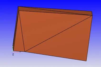
- flagging
- flag the boundaries as shown below

- flag the boundaries as shown below
- Check diagnostics
- As per diagnosis result it seems like there are no errors.
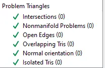
- As per diagnosis result it seems like there are no errors.
- Start case setup
- Application type: Time based
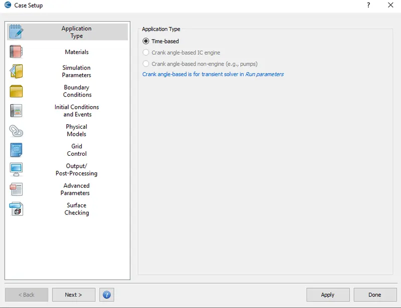
- Materials
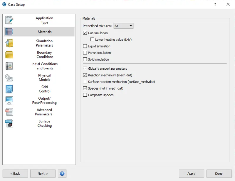
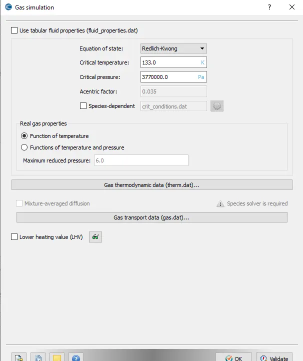
- Gas simulation: let everything set to default value.
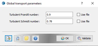
- Global transport parameter
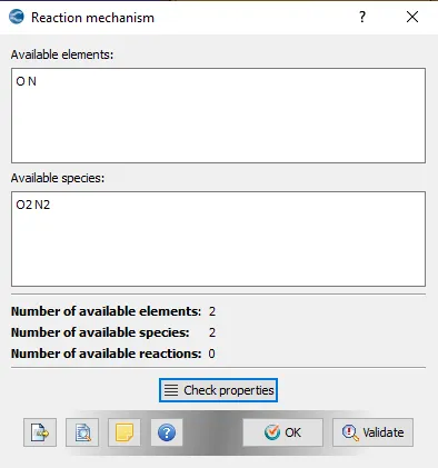
- Reaction mechanism
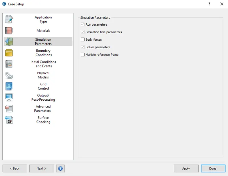
- Simulation parameter
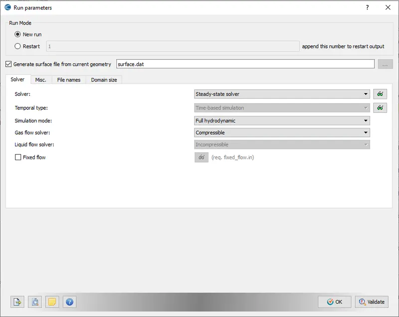
- Run parameters
- solver type: steady-state solver
- simulation mode: full hydrodynamic
- gas flow solver: compressible
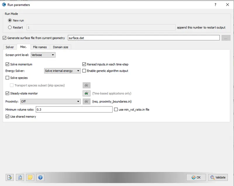
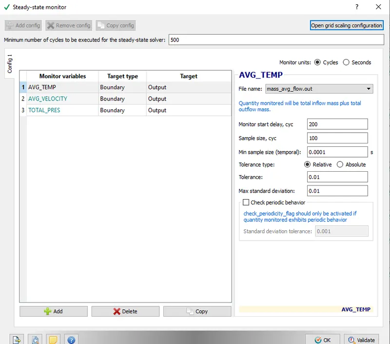
- Steady state monitor
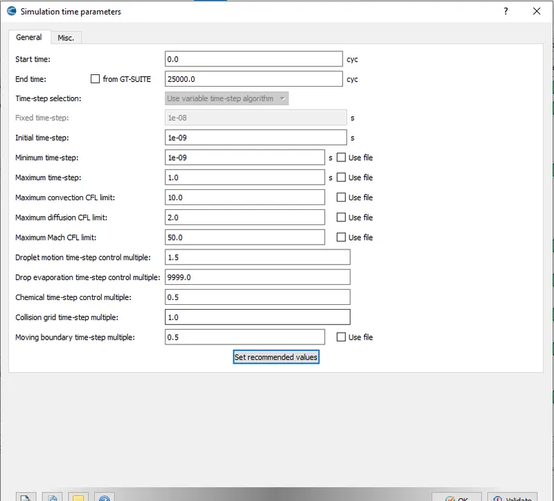
- Simulation time parameter
- start time: 0 cycles.
- end time: 25000 cycles.
- initial time step: 1e-9 sec.
- minimum time step: 1e-9 sec.
- maximum time step: 1 sec.
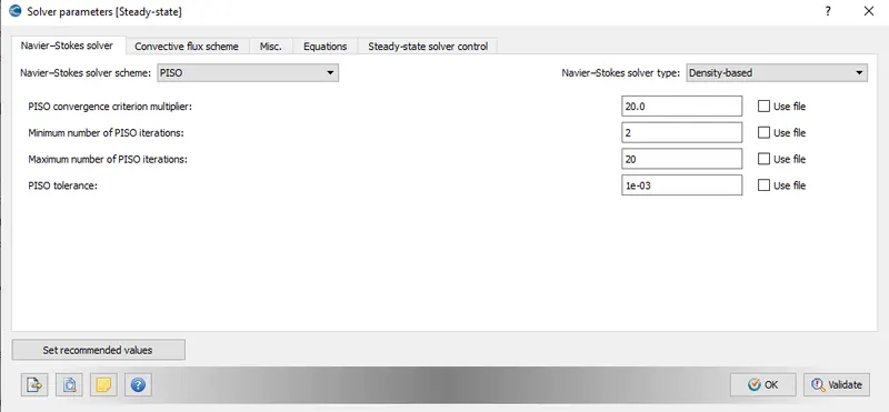
- Solver parameters
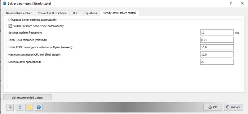
- Boundary conditions
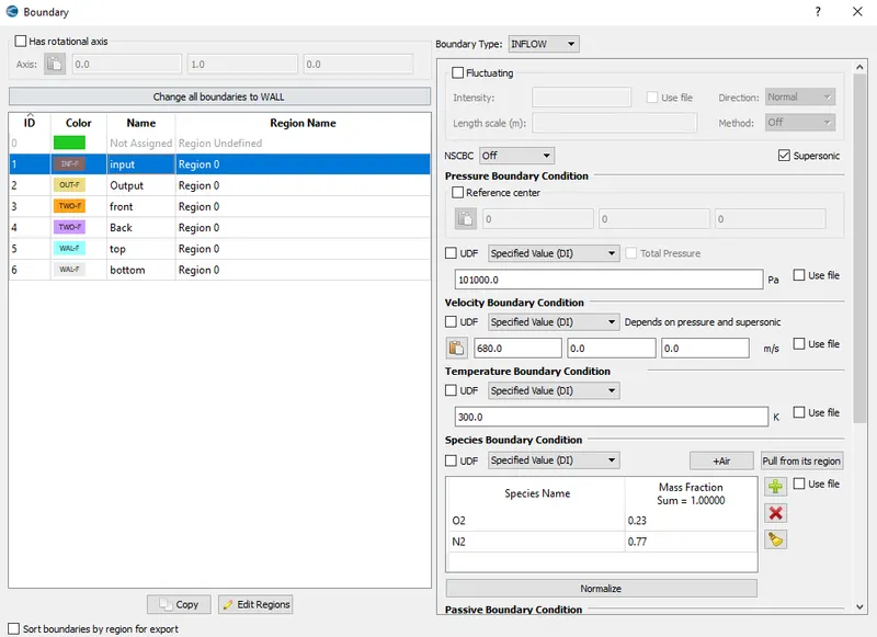
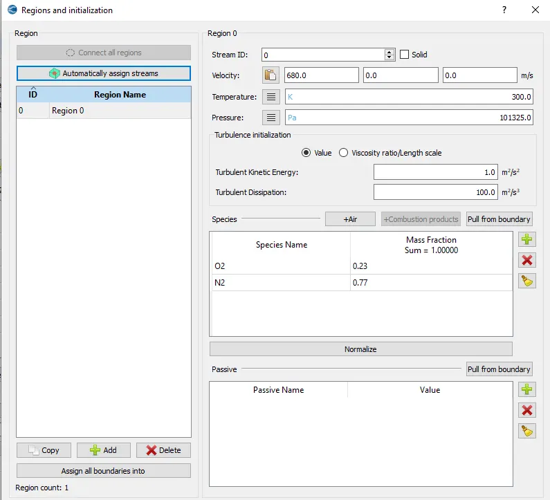
- Inlet
- Boundary type: inflow
- pressure boundary condition: 101000 Pa
- Temperature boundary conditions: 300K
- Velocity boundary conditions: 680m/sec
- Species boundary condition: Air
- Outlet
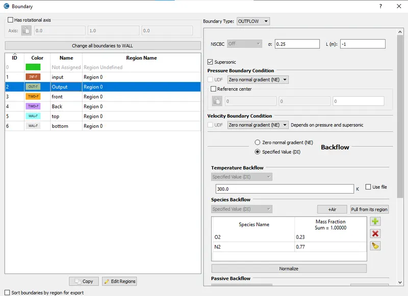
- Boundary type: outflow
- pressure boundary condition: Neumann boundary condition
- Temperature boundary conditions: 300K
- Velocity boundary conditions: Neumann boundary condition
- Species boundary condition: Air
- Front
- Boundary type: 2D
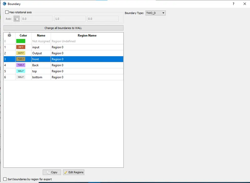
- Boundary type: 2D
- Back
- Boundary type: 2D
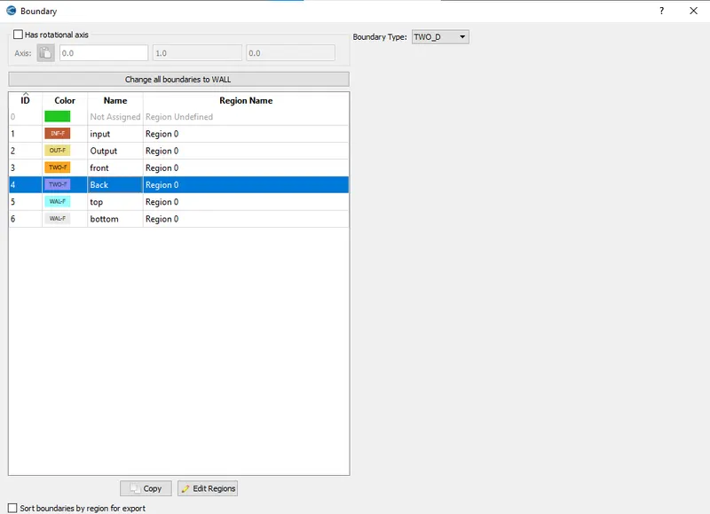
- Boundary type: 2D
- Top Wall
- Boundary type: wall
- velocity boundary condition:
- wall motion type: stationary
- surface movement: FIXED
- Slip
- Temperature boundary condition: Neumann boundary condition.
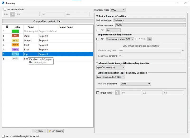
- Bottom Wall
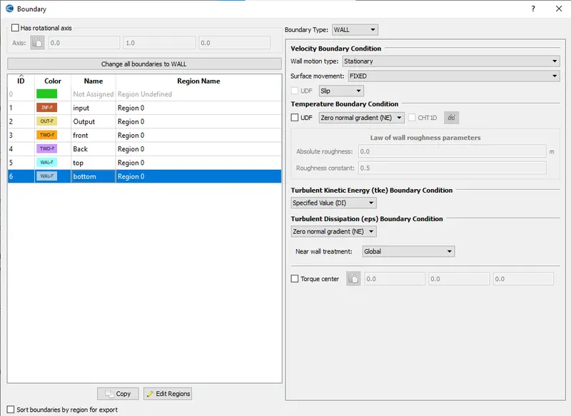
- Boundary type: wall
- velocity boundary condition:
- wall motion type: stationary
- surface movement: FIXED
- Slip
- Temperature boundary condition: Neumann boundary condition.
- Inlet
- Regions and initializations
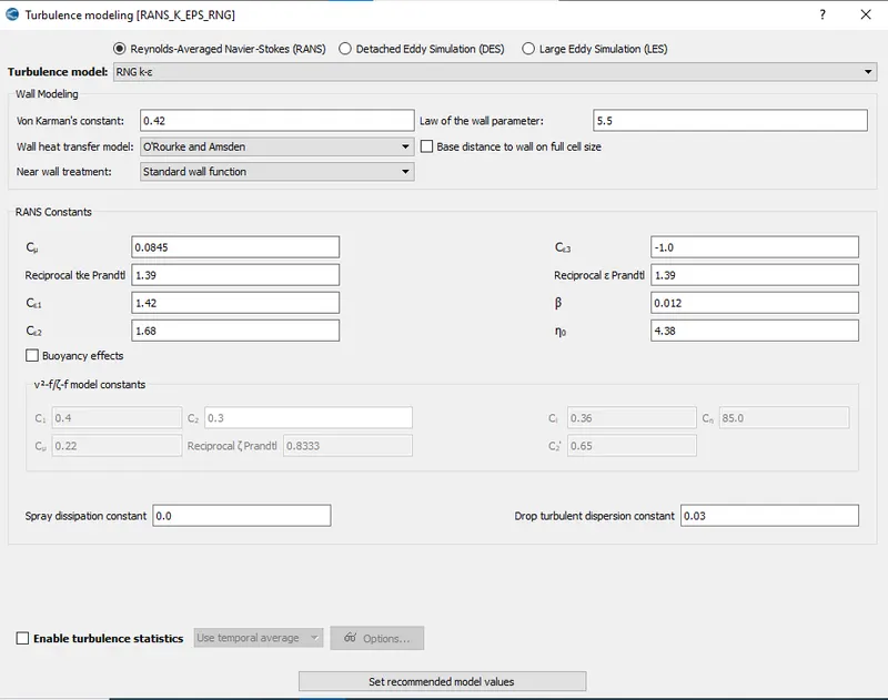
- Turbulence model
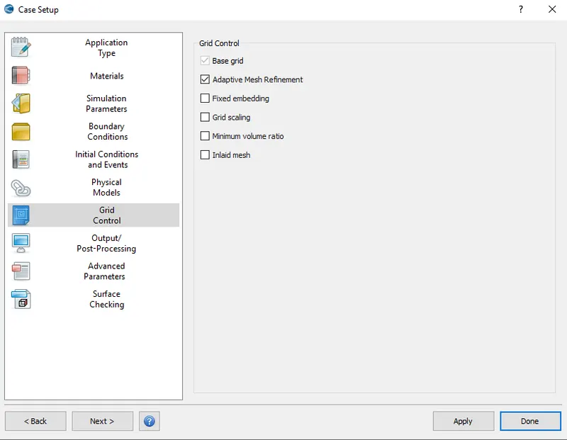
- Grid control
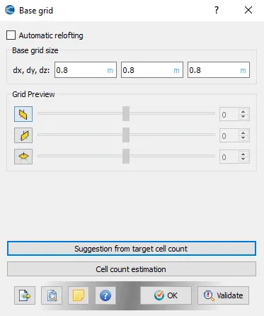
- Base grid
- Adaptive mesh refinement
- sub rid criterion was taken 0.05 and 0.01K in two different cases.
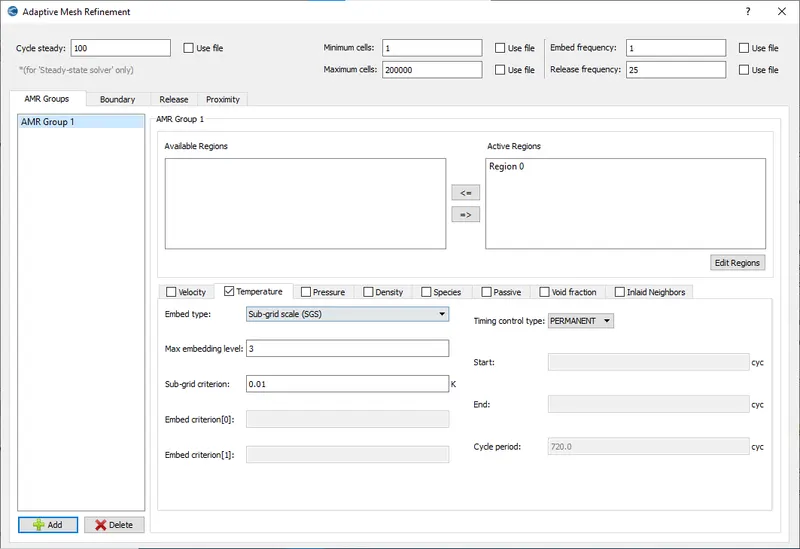
- sub rid criterion was taken 0.05 and 0.01K in two different cases.
- Base grid
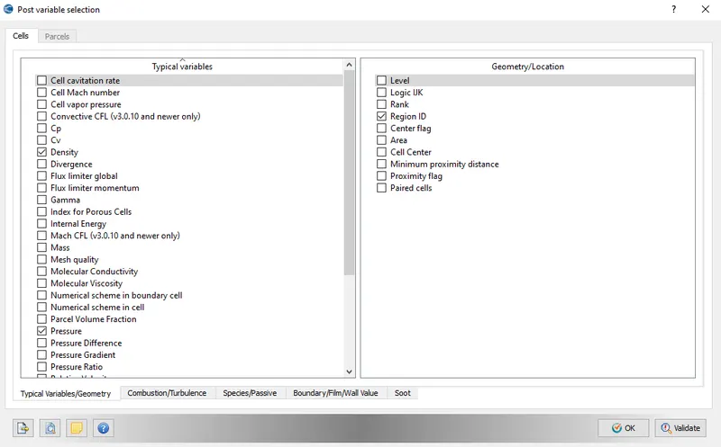
- Post variable selection
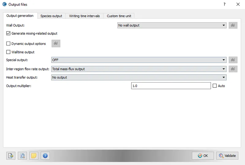
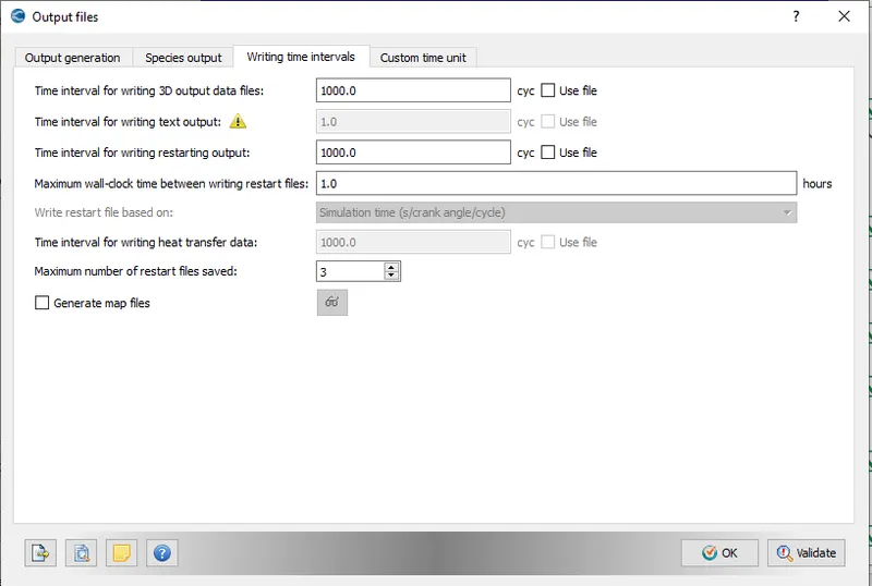
- Output variables
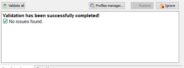
- Validate the setup before exporting.
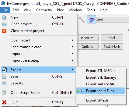
- Export the case setup
Result and Outputs
Case-I for SGS value of 0.001
Mesh profile for SGS value 0.001
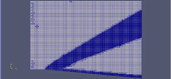
Mesh size of 0.8 m along all directions with the adaptive mesh refinement of 0.001. we can observe the AMR with blue colored mesh.
Temperature contour for SGS Value 0.001
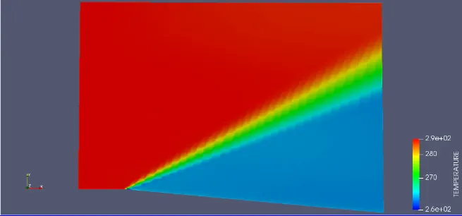
The temperature contour shows the formation of the expansion fan at the expansion point.
Velocity contour for SGS value 0.001
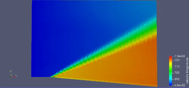
The velocity contour shows the formation of the expansion fan at the expansion point.
Pressure contour for SGS 0.001
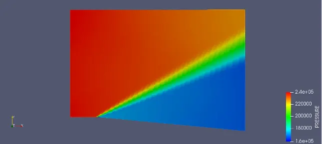
The pressure contour shows the formation of the expansion fan at the expansion point.
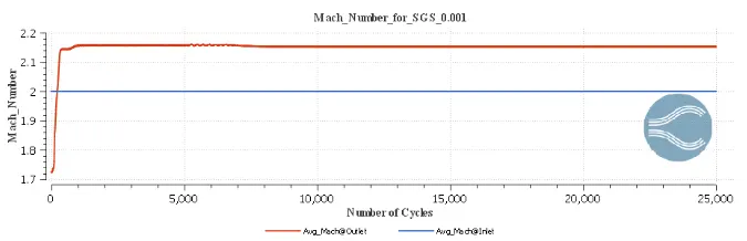
Plot for average Mach no. vs cycle
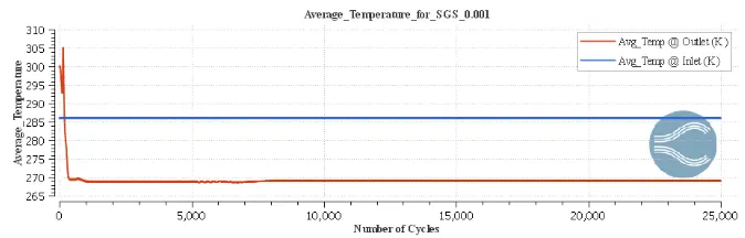
Plot for average temperature vs cycle
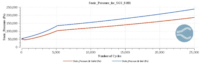
Plot for Static pressure vs no. of cycles
Total cells vs cycles
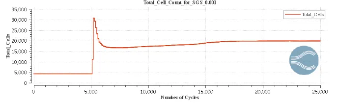
- The total cells in this case are around 20000. and the solution converged after 20000 cycles and it is a steady state simulation.
- the Mach no. of the flow is increasing after passing through the expansion fan and the remaining properties like static pressure, temperature is declined.
Case II for SGS value of 0.01
Mesh profile for SGS value 0.01
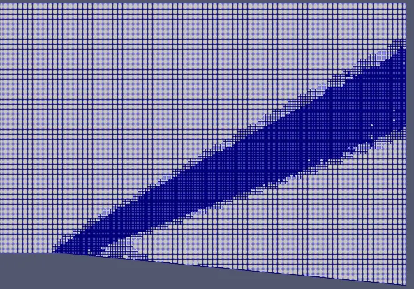
Mesh size of 0.8 m along all directions with the adaptive mesh refinement of 0.01.
Temperature contour for SGS Value 0.01
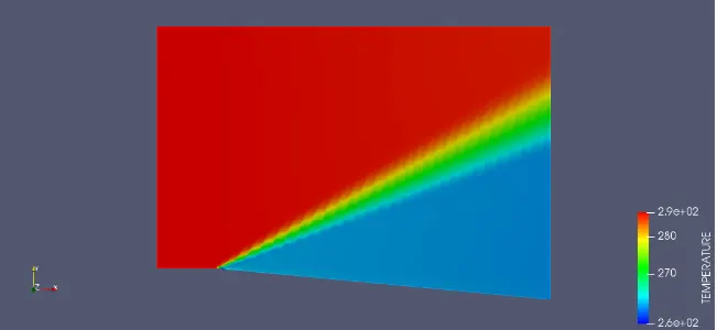
The temperature contour shows the formation of the expansion fan at the expansion point.
Velocity contour for SGS value 0.01
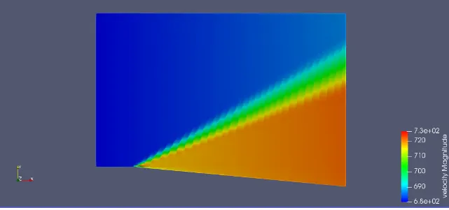
The velocity contour shows the formation of the expansion fan at the expansion point.
Pressure contour for SGS 0.01
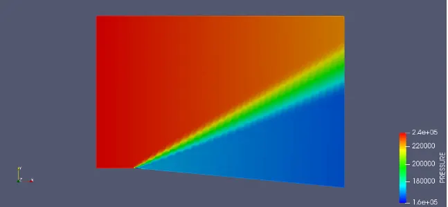
The pressure contour shows the formation of the expansion fan at the expansion point.
Plot for average Mach no. vs cycle
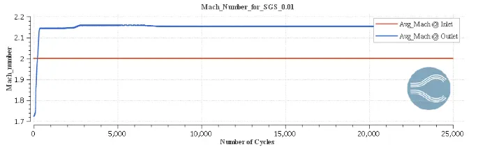
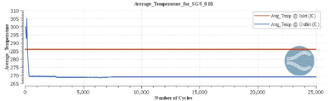
Plot for average temperature vs cycle
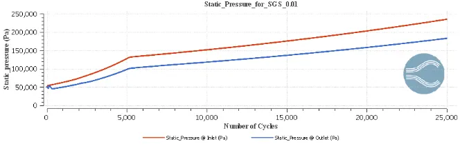
plot for Static pressure vs no. of cycles
Total cells vs cycles
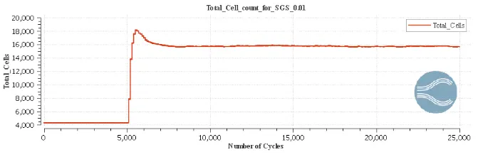
- The total cells in this case are around 16000. and the solution converged after 14000 cycles and it is a steady state simulation.
- the Mach no. of the flow is increasing after passing through the expansion fan and the remaining properties like static pressure, temperature is declined.
Case III for SGS value of 0.1
Mesh profile for SGS value 0.1
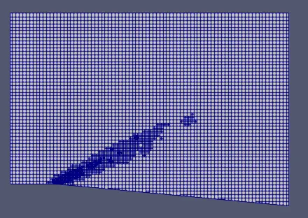
Mesh size of 0.8 m along all directions with the adaptive mesh refinement of 0.1.
Temperature contour for SGS Value 0.1
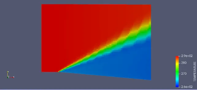
The temperature contour shows the formation of the expansion fan at the expansion point.
Velocity contour for SGS value 0.1
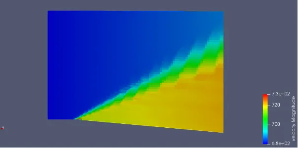
The velocity contour shows the formation of the expansion fan at the expansion point.
Pressure contour for SGS 0.1
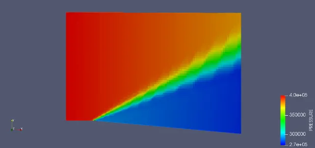
The pressure contour shows the formation of the expansion fan at the expansion point.
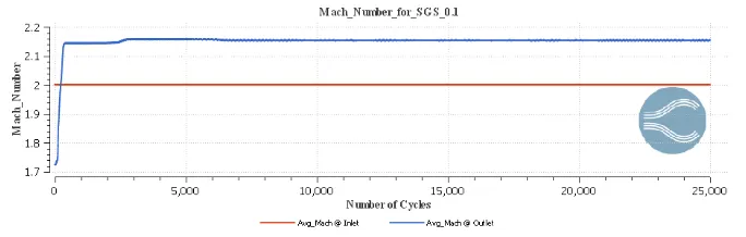
Plot for average Mach no. vs cycle
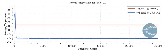
Plot for average temperature vs cycle
plot for Static pressure vs no. of cycles
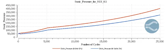
Total cells vs cycles
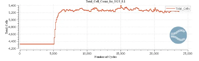
- The total cells in this case are around 5200-5400. and the solution converged after 20000 cycles and it is a steady state simulation.
- the Mach no. of the flow is increasing after passing through the expansion fan and the remaining properties like static pressure, temperature is declined.
Effect of SGS on total cell count
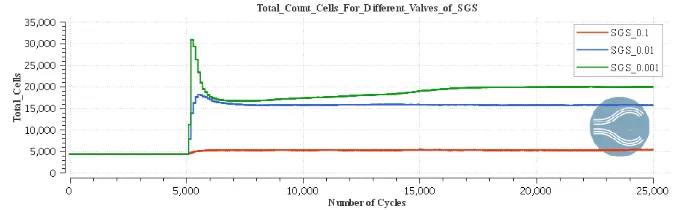
- From the above plot we can observe that the more we decrease the SGS value the more the mesh will be refined and no. of cell count will increase.
Conclusion
- Different values of SGS were performed during the project and it was observed that as we decrease the SGS value mesh get more refined.
- With the fine mesh, we can clearly observe the expansion fan with a little width.