Week 5: Prandtl Meyer Shock problem
Prandtl Meyer Shock problem
Shock Wave:
Shock is an abrupt discontinuity in the flow field and it occurs inflows when the local flow speed exceeds the local sound speed. More specifically, it is a flow whose Mach number exceeds 1.
A shock wave is a type of propagating disturbance that moves faster than the local speed of sound in the medium. Like an ordinary wave, a shock wave carries energy and can propagate through a medium but is characterized by an abrupt, nearly discontinuous, change in pressure, temperature, and density of the medium.
When an object is moving in a flow field the object sends out disturbances that propagate at the speed of sound and adjusts the remaining flow field accordingly. However, if the object itself happens to travel at speed greater than sound, then the disturbances created by the object would not have traveled and communicated to the rest of the flow field and this results in an abrupt change of property, which is termed as a shock in gas dynamics terminology.
Shocks are characterized by discontinuous changes in flow properties such as velocity, pressure, temperature, etc. Typically, shock thickness is of a few mean free paths(of the order of 10−8 m). Shocks are irreversible occurrences in supersonic flows.
Shock types:
- Normal shock:
- Normal shocks are generally 90* perpendicular to the direction of the shock flow medium.
- Oblique shock:
- When the flow field is still attached to the body, the shock wave which is deviating at some arbitrary angle from the flow direction is termed oblique shock.
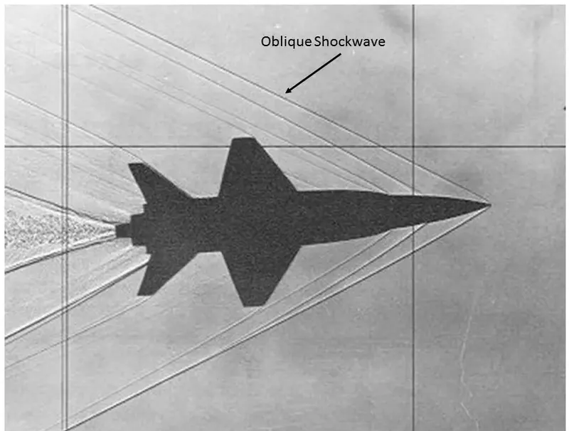
- Bow shock:
- When an oblique shock is likely to form at an angle that cannot remain on the surface, a nonlinear phenomenon arises where the shock wave will form a continuous pattern around the body. These are termed bow shocks.
Prandtl–Meyer expansion fan:
Prandtl–Meyer expansion fan, a two-dimensional simple wave, is a centered expansion process that occurs when a supersonic flow turns around a convex corner. The fan consists of an infinite number of Mach waves, diverging from a sharp corner. When a flow turns around a smooth and circular corner, these waves can be extended backward to meet at a point.
Each wave in the expansion fan turns the flow gradually (in small steps). It is physically impossible for the flow to turn through a single "shock" wave because this would violate the second law of thermodynamics. Across the expansion fan, the flow accelerates (velocity increases) and the Mach number increases, while the static pressure, temperature, and density decrease. Since the process is isentropic, the stagnation properties (e.g. the total pressure and total temperature) remain constant across the fan.
Shock flow boundary conditions:
Boundary conditions (b.c.) are constraints necessary for the solution of a boundary value problem. A boundary value problem is a differential equation (or system of differential equations) to be solved in a domain on whose boundary a set of conditions is known.
Both ordinary and partial differential equations need boundary conditions to be solved. Different types of boundary conditions can be imposed on the boundary of the domain. The choice of the boundary condition is fundamental for the resolution of the computational problem: a bad imposition of b.c. may lead to the divergence of the solution or to the convergence to a wrong solution.
There are five types of boundary conditions. From in Fluid mechanics point of view, we use the first 3 boundary conditions.
- Dirichlet boundary condition:
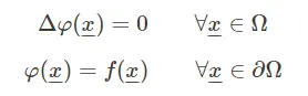
- This condition specifies the value that the unknown function needs to take on along the boundary of the domain. Given, for example, the Laplace equation, the boundary value problem with the Dirichlet b.c. is written as:
-
-
The classical Dirichlet boundary condition consists of the value of velocity and/or pressure to be taken by a certain set of nodes. It is common to refer to some sets of b.c. according to the following terminology:
- slip boundary condition: the velocity normal to the boundary is set to zero, while the velocity parallel to the boundary is let free
- no-slip boundary condition: both the velocity normal to the boundary and the velocity parallel to the boundary are set equal to zero.
At least one homogeneous b.c. on the pressure (i.e. p=0) has to be imposed as a reference for open domains, for instance, in the highest boundary of the air domain.
- where φ is the unknown function, x_ is the independent variable (e.g. the spatial coordinates), Ω is the function domain, ∂Ω is the boundary of the domain, and f is a given scalar function defined on ∂Ω.
- Neumann boundary condition:
- When imposed on an ordinary (ODE) or a partial differential equation (PDE), it specifies the values that the derivative of a solution is going to take on the boundary of the domain.
-
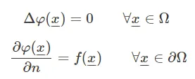
- Constraints on the derivative of velocity or pressure fields are mainly used in two cases. The first case is the application of a symmetry plane, thus:
-

- Since this condition is always applied in addition to a Dirichlet b.c. it is naturally satisfied. The second application is the modeling of wall friction, in the case when it is proportional to the strain rate:

- Robin boundary condition:
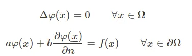
- It consists of a linear combination of the values of the field and its derivatives on the boundary.
- Since this condition is always applied in addition to a Dirichlet b.c. it is naturally satisfied. The second application is the modeling of wall friction, in the case when it is proportional to the strain rate:
- Mixed boundary condition:
- It consists of applying different types of boundary conditions in different parts of the domain. It is important to notice that boundary conditions must be applied on the whole boundary: the “free” boundary is anyways subjected to a homogeneous Neumann condition. The mixed boundary condition differs from the Robin condition because the latter consists of different types of boundary conditions applied to the same region of the boundary, while the mixed condition implies different types of b.c. applied to different parts of the boundary.
- Cauchy boundary condition:
- The Cauchy boundary condition is a condition on both the unknown field and its derivatives. It differs from the Robin condition because the Cauchy condition implies the imposition of two constraints (1 Dirichlet b.c. + 1 Neumann b.c.), while the Robin condition implies only one constraint on the linear combination of the unknown function and its derivatives.
BC's are typically used for shock flow problems:
In this shock wave problem, we have to use the Neumann boundary condition. Since this condition is always applied in addition to a Dirichlet b.c.
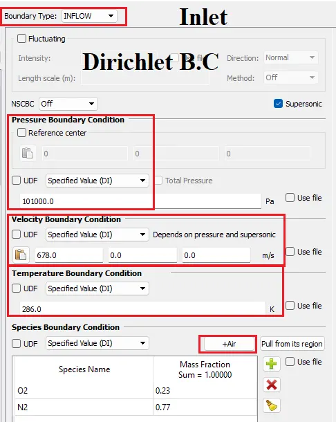
For Inlet, we are going to use Dirichlet boundary conditions for all parameters like Pressure, Velocity, and Temperature.
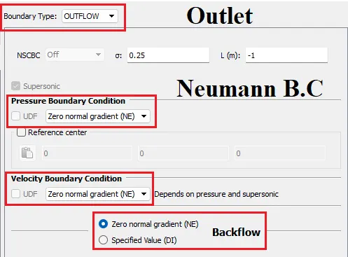
For Outlet, we should assign Neumann boundary conditions for all parameters like Pressure, Velocity, and Temperature.
My Own Words on the Dirichlet & Neumann Boundary conditions:
In Dirichlet B.C we will specify the magnitudes of the variable in the form of scalers or vectors at the particular boundary face. Ex: Pressure, Velocity, Temperature, and Heat flux can be specified at the inlet.
In Neumann B.C we will specify magnitudes of the variables in the form of a Normal gradient. In this case, we don't need to specify values near the boundary faces, based on the Normal derivative assigned and the domain interface codes will automatically calculate the magnitude of the variable at the boundary.
Ex: Zero Normal Gradient means zero difference between the magnitude of any variable in the cell or node attached to the boundary face and the cell which is attached to the boundary cell.
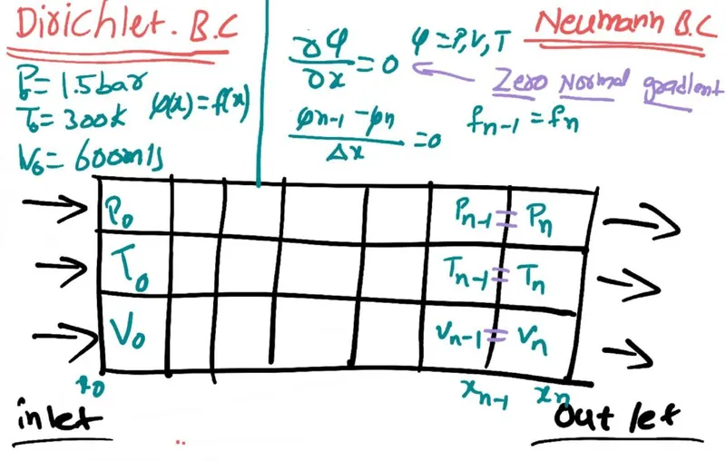
Why Neumann Boundary Condition Used in Shock Flow problem:
Basically, Shock flows are supersonic flows with a Mach number greater than 1. For this kind of situation, it is difficult to interpolate the results i.e, we use Neumann B.C for shock flow problems.
Flow simulation in CONVERGE done in 3 steps:
- Geometry preparation and Case setup :
- We use Converge GUI(Graphical User Interface) to set up the case and export input files.
- Solving the problem using input files:
- These input files are solved by Converge in the Terminal (Command-line interface). We USed Cygwin for the command line terminal.
- Post-processing results:
- We convert our solution into Paraview binary format to post-process the results in Paraview
Geometry preparation in CONVERGE CFD:
- Geometry preparation:
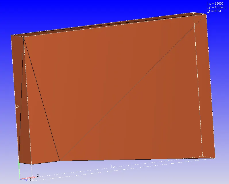
- Import the ".STL" for Prandtl Meyer shock problem simulation.
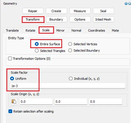
- Scaling the Geometry.
- In Converge default units are in meters. So, we have to scale the geometry by scaling factor 0.001 to convert it into a proper scale.
- Transform => Scale => Entire Surface => Scale factor = 0.001
- Import the ".STL" for Prandtl Meyer shock problem simulation.
- Boundary Flagging:
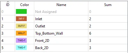
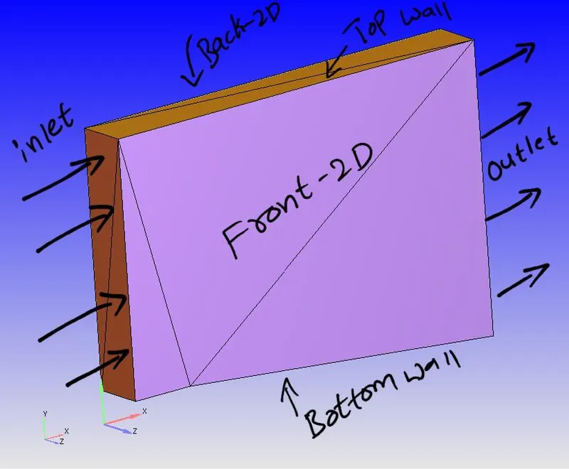
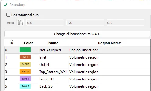
- We have to flag Inlet, Outlet, Top_Bottom_walls, Front & Back faces boundaries for the above-created geometry.
- By default In CONVERGE, all the surfaces are made up of triangles we have to select respective triangle faces for flaging.
- Boundary => Flag
- Normal Transformation:
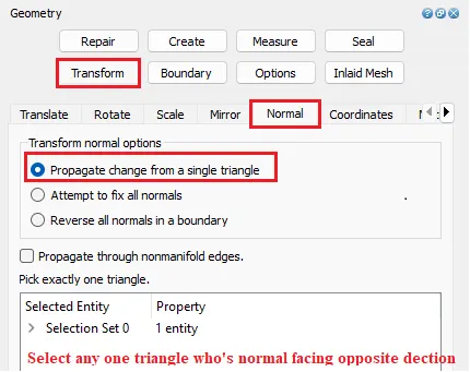
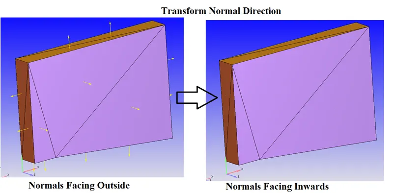
- All the face normals directions should be facing towards the flow region.
- In this fluid is flowing through the channel but normals are facing outwards. We have to transform the normal's direction.
- Diagnosis:
- Checking for any interactions, open edges, etc.
Case Setup in CONVERGE CFD:
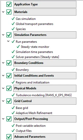
| 1 | Application Type | Time-based |
| 2 | Materials | |
| Gas simulation | Default | |
| Global transport properties | Default | |
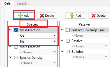
| Species | Add:- O2, N2 | |
| 3 | Initial Conditions and Events | |
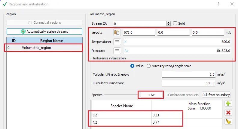
| Regions and initializations | Add:- Volumetric region, V = 678 m/s, T = 300K, P = 1 bar | |
| 4 | Boundary Conditions | |
| Boundary | ||
| Simulation Parameters | ||
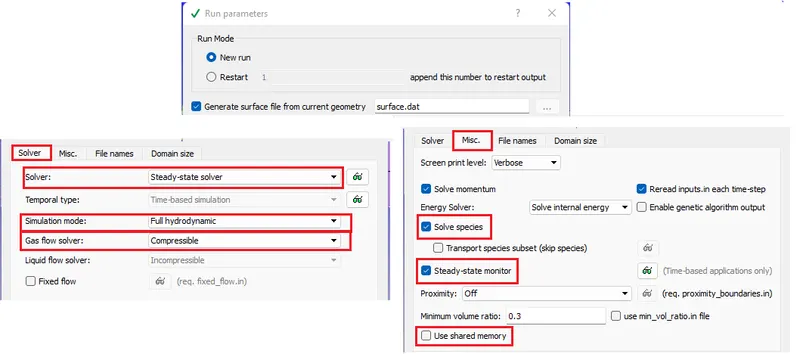
| Run parameters | Steady State solver, Fully hydrodynamic, Compressible,Ste | |
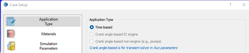
- Application Type :
- Materials:
- Set default values in Gas Simulation & Global transport parameters.
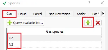
- Species: Add Gas species O2 & N2.
- Initial Conditions and Events:
- Add Volumetric region in region section.
- We have to give the initial condition (initial state) to the flow domain. Good initial condition helps the solution to converge quickly and to get good results.
- Boundary conditions:
- Defining boundary type and conditions:
-
Boundary Name Type Boundary Condition Pressure Velocity Temperature Species Inlet INFLOW Dirichlet 101000 Pa 678 m/s 286k O2 : 0.23 & N2 : 0.77 Outlet OUTFLOW Neumann Zero normal gradient Zero normal gradient Zero normal gradient O2 : 0.23 & N2 : 0.77 Top_Bottom_walls WALL Slip Front_2D TWO_D Back_2D TWO_D - INLET: Since it’s a supersonic flow at the inlet we should assign Dirichlet boundary conditions for all parameters like Pressure, Velocity, and Temperature. So, We can give Static pressure= 101000 Pa, Velocity=678m/s and Temperature=286k
- OUTLET: At the outlet, we should assign Neumann boundary conditions for all parameters like Pressure, Velocity, and Temperature. So, We can give a Zero normal gradient for all the parameters.
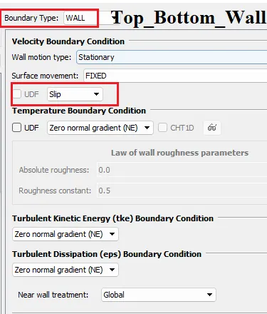
- Top_Bottom_walls:
- Since the supersonic flow is inviscid in nature(the viscous effect is negligible) we can assume the Slip condition at the wall.
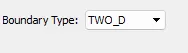
- FRONT_2D & BACK_2D: The 2D planar assumption is used because the flow gradients along the z-direction are negligible when compared to the other two directions. By reducing the model to 2D, the Prandtl Meyer can be simulated and analyzed cost-effectively compared to a full 3D model.
- INLET: Since it’s a supersonic flow at the inlet we should assign Dirichlet boundary conditions for all parameters like Pressure, Velocity, and Temperature. So, We can give Static pressure= 101000 Pa, Velocity=678m/s and Temperature=286k
- Defining boundary type and conditions:
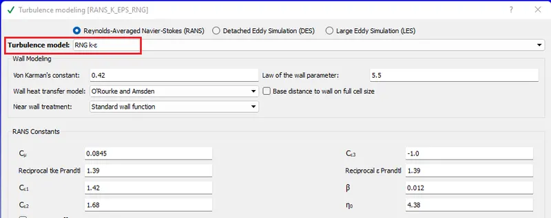
- Turbulence Modelling: No need for the Turbulence model.
Reason: In our simulation, we don't have to use Turbulence modeling since there is no Reynolds stress because the flow is inviscid. - Simulation Parameters:
- Run Parameters:
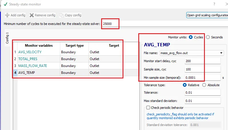
- Selecting the Solver & solver type. informing additional things to solve (Energy & Momentum equations) and monitoring steady-state.
- Steady-state monitor:
- In this, we have to Add monitor variables to be monitored during the simulation at different boundaries.
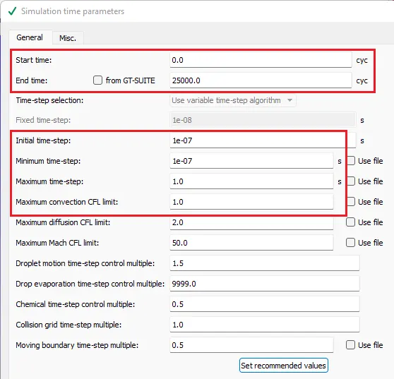
- Simulation Parameter:
- defining initial, Minimum & Maximum Time step sizes.
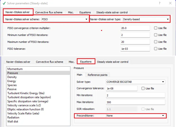
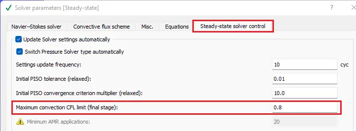
- Solver Parameters:
- Solver Scheme to PISO and Density-based solver.
- under Equations window set precondition to None for all the variables.
- Run Parameters:
- Physical Models:
- usingRenoulds Average Navier stroke equation
- usingRenoulds Average Navier stroke equation
- Grid Control:
- This is the section where we define meshing.
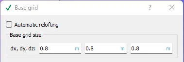
- Base grid:
- Adaptive Mesh refinement (AMR):
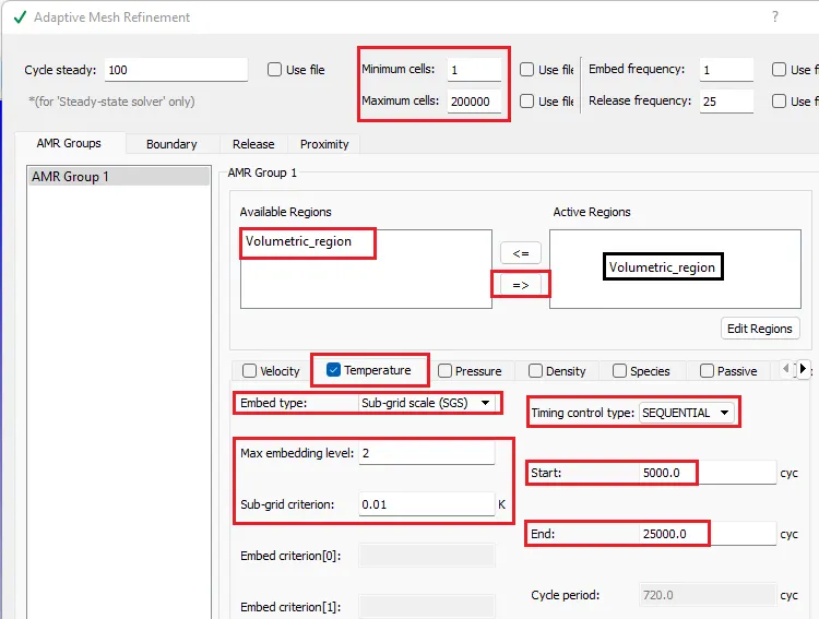
- In Adaptive Mesh refinement mesh gets auto-refined according to the condition given.
- here we are specifying the maximum number of cells that can be reached after refinement is 200,000 cells.
- firstly we have to shift the Volumetric_region in available regions to active regions.
- For this case, we are using temperature-based AMR so that we can monitor curvature in temperature. whenever the curvature of the temperature is greater than the particular value we refine the mesh.
- Embed type: Sub-grid Scale (SGS)
- we have to enter magnitude for sub-grid criterion. for example, if we enter Sub-grid criterion = 0.1 K mesh gets auto refined in the region where the temperature difference between `N_(th)` cell and N-1 cell is greater than the criteria.
- Max embedding level is used to calculate and refine the mesh to the maximum possible limit(minimum size).
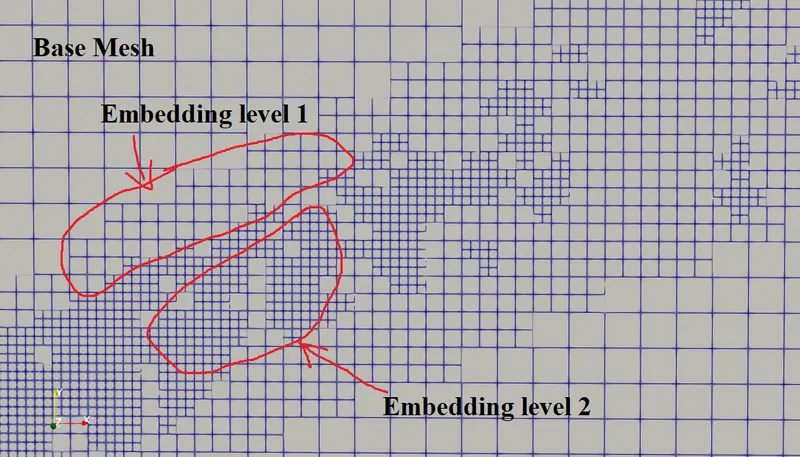
- `text(Grid size) = (text(Base grid size))/2^text(Embed level)`
- For this simulation, we used base grid size = 0.8m and embed level = 2
- `text(Smallest possible cell size) = 0.8/2^2=0.8/4=0.2 m`
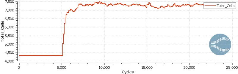
- We don't need mesh refinement right from the beginning of the simulation because at the being we have lot of residuals in the solution. we can refine the mesh after 5000 cycles.
- Output/Post-Processing
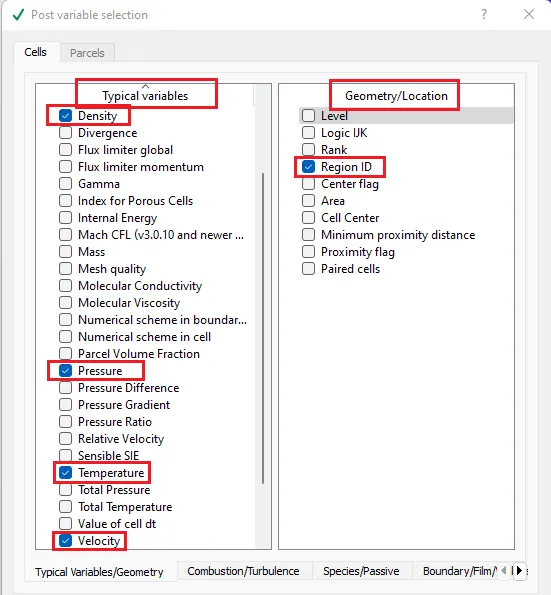
- Post Variable selection: select the variables to be monitored for post-processing.
- Post Variable selection: select the variables to be monitored for post-processing.
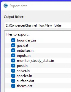
- Exporting Input files:
- Export the input files
- Export the input files
Solving Channel Flow in Cygwin:
- Go to the directory where input files are exported
- Make mpiexec.exe & converge.exe files globally available.
- "mpiexec.exe -n 4 converge.exe restricted </dev/null> logfile &"
- Use above mentioned line to start calculation in the background
- mpiexec.exe & converge.exe are executable applications to solve the problem
- -n 4:- number of processors
- restricted:- my license is a restricted one.
- </dev/null> logfile:- creates temporary memory to save data with name as logfile at a particular iteration
- & :- To run Calculation in Background
- "tail -10 logfile" command is used to view the last 10 lines of the logfile.
- "mpiexec.exe -n 1 post_convert_30_serial_64" command used to convert output files to paraview binary format, so that they can be processed in the paraview.
Post Processing and Results from Paraview:-
- open "..vtm" group file in paraview. This group contains all the solution files.
- use the slice tool to create a contour section plane and plot the contours
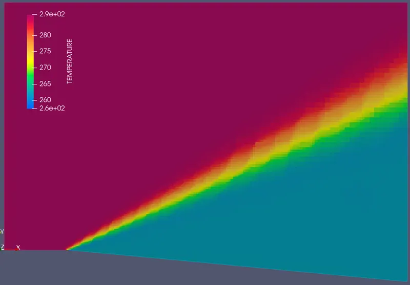
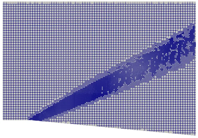
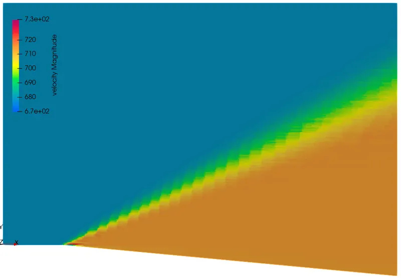
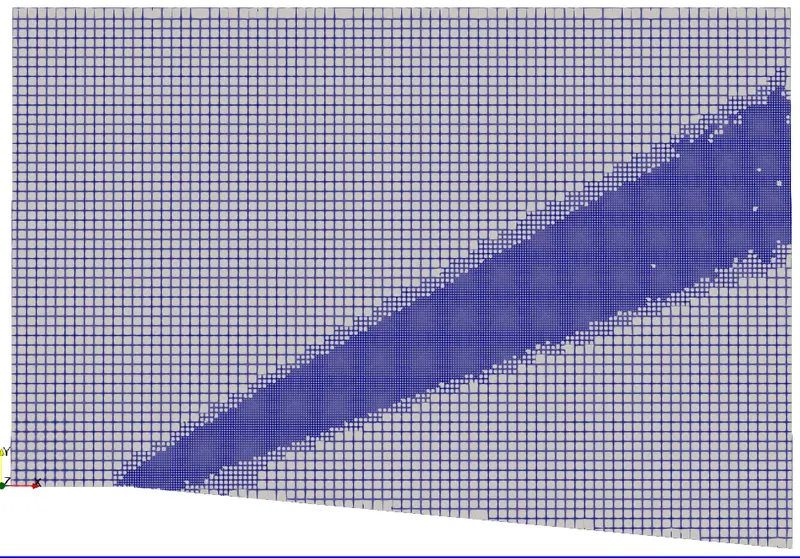
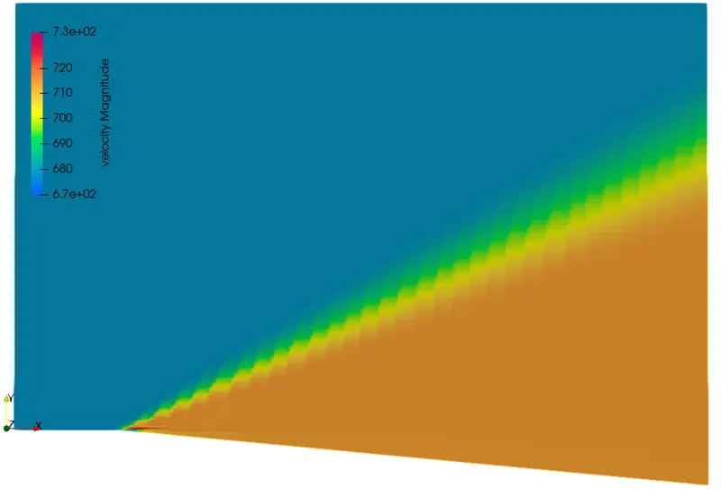
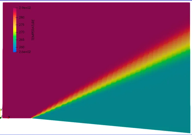
- Case 1: Temperature Subgrid criterion = 0.05 K
- Mesh
- Velocity Contour
- Temperature Coutour
- Plots:
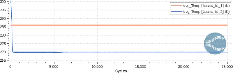
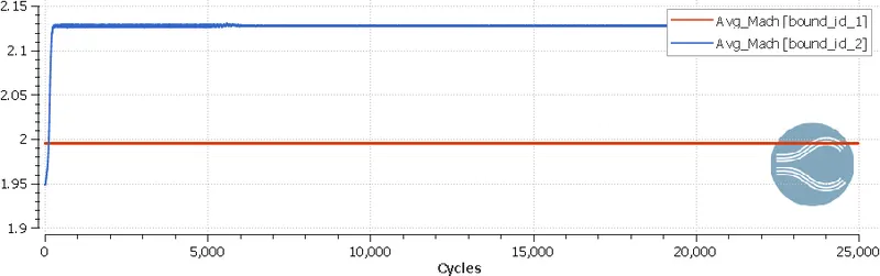
- bound_id_1 = inlet
- bound_id_2 = outlet
- Mesh
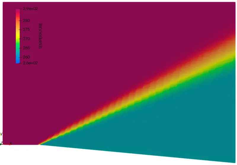
- Case 2: Temperature Subgrid criterion = 0.025 K
- Mesh
- Velocity Contour
- Temperature Coutour
- Plots
- bound_id_1 = inlet
- bound_id_2 = outlet
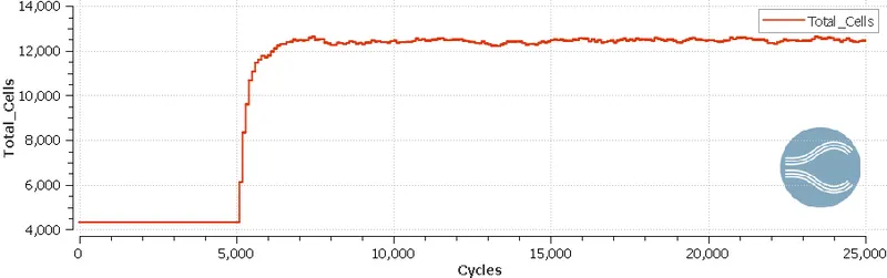
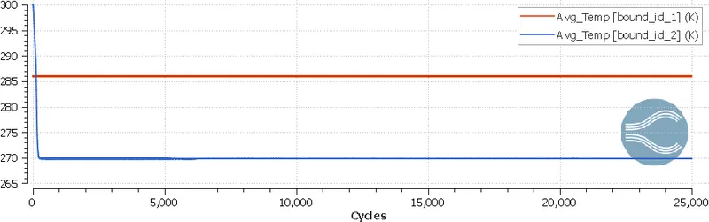
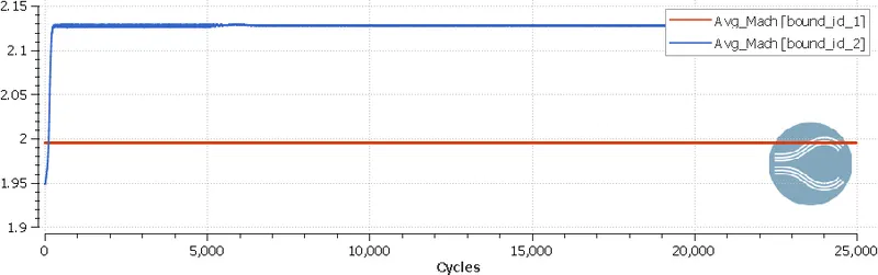
- Mesh
- Case 3: Temperature Subgrid criterion = 0.01 K
- Mesh
- Velocity Contour
- Temperature Coutour
- Plots
- bound_id_1 = inlet
- bound_id_2 = outlet
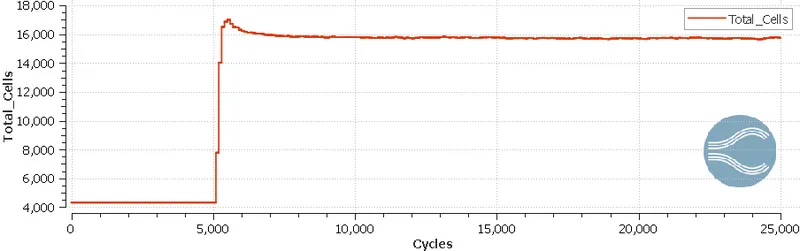
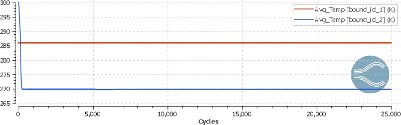
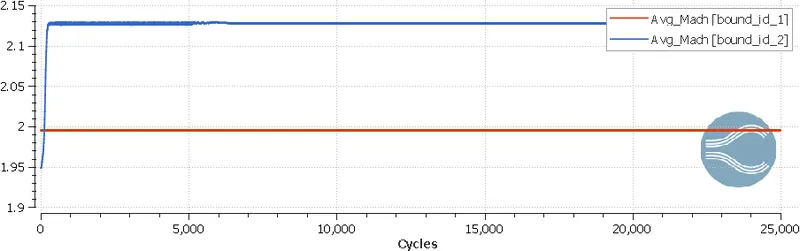
- Mesh
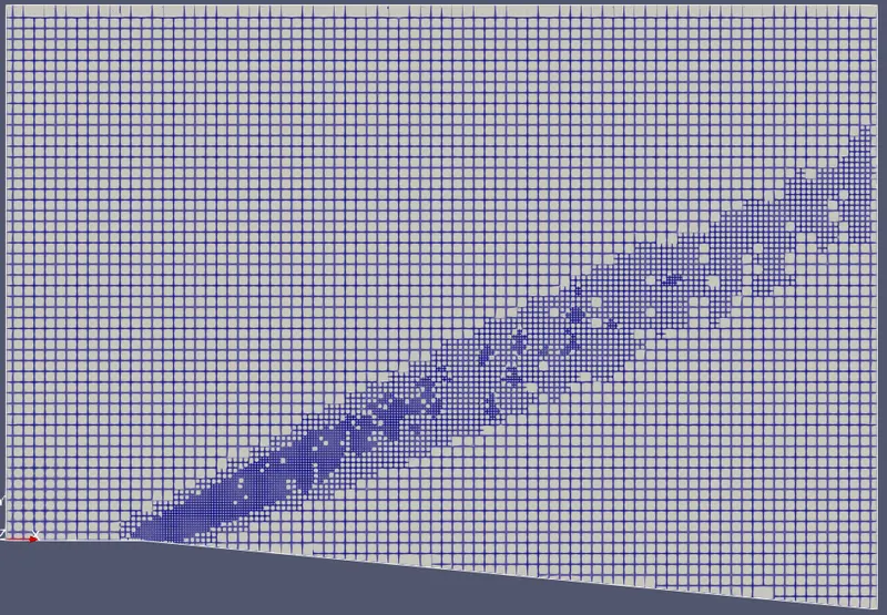
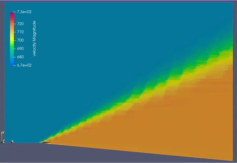
Result Table:
| Base mesh dx=dy=dz= | Temperature Sub Grid Scale | Final Cell count | Simulation time (seconds) | Mass flow rate(Kg/s) | Mach number | Pressure (Pa) | Temperature K | |||||
| (m) | Inlet | Outlet | Inlet | Outlet | Inlet(Static) | Outlet(Static) | Inlet | Outlet | ||||
| Case_1 | 0.8 | 0.05 | 7319 | 549.68 | 33240 | 33240.6 | 1.995 | 2.127 | 101000 | 82610.3 | 286 | 269.83 |
| Case_2 | 0.8 | 0.025 | 12452 | 802.95 | 33240 | 332398.7 | 1.995 | 2.127 | 101000 | 82631.1 | 286 | 269.83 |
| Case_3 | 0.8 | 0.01 | 15760 | 1018.55 | 33240 | 33239.9 | 1.995 | 2.127 | 101000 | 82650.8 | 286 | 269.85 |
Conclusion:
- When we compare the temperature contours & Mesh for three different cases we can observe more refinement as the subgrid criteria decrease.
- In the first case, mesh gets refined when the temperature difference in `n_(th)`cell and `n-1_(th)` is greater than 0.05 for the second and third case mesh gets refined when the difference is greater than 0.025 & 0.01 respectively.
- As the mesh gets refined cell count increases in a particular region to capture more details for good results.
- Sub-grid-scale refinement is more useful when we need local refinement based on thermodynamic properties changing beyond the limit.
- From Total_cell plots We can observe as the solutions advance there is a fluctuation in total cell count. As the Sub-Grid value decreases the amplitude of the fluctuations also decreases and is maintained at a relatively constant level.
https://www.simscale.com/docs/simwiki/numerics-background/what-are-boundary-conditions/