Solving the steady and unsteady 2D heat conduction problem

Introduction

In this project, the 2D heat conduction equation is simulated and studied using implicit and explicit schemes for steady and unsteady conditions using MATLAB.

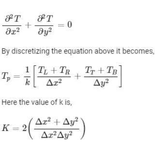
`(delT)/(delt) + alpha((del^2T)/(delx^2) + (del^2T)/(dely^2) ) = 0`

The steady state form of this equation would be:

`alpha((del^2T)/(delx^2) + (del^2T)/(dely^2) ) = 0`

Three iterative solvers will be used for the transient and steady cases:

1. Jacobi
2. Gauss Seidel
3. Succesive over relaxation

Note: During the discretization explaination steps, nodes at (i-1,j), (i+1,j),(i,j+1) and (i,j-1) will be reffered to as left, right, top and bottom respectively.

Code and logic

First, the steady and unsteady equations are converted from their differential forms to analytical forms using finite difference schemes. (2nd order central differencing).

Every Solver is defined as a seperate function and called into the code when required for each condition.

Boundary conditions are assigned and inputs are defined as seen in steps 1 and 2.

Boundary conditions for the temperature domain:

Top Boundary = 600 K

Bottom Boundary = 900 K

Left Boundary = 400 K

Right Boundary = 800 K

The main code is as follows:

clear all
close all
clc


%STEP 1 -----------------------------> CREATING THE GRID POINTS AND INPUTS
alpha = 1.4;
nx = 10;
ny = nx;
x = linspace(0,1,nx);
dx = x(2)-x(1);
y = linspace(0,1,ny);
dy = y(2)-y(1);
tolerance = 1e-4;
error = 9e9;
k = 2*((dx^2 + dy^2)/(dx^2*dy^2));
dt = 300;
nt = 1400;
k1 = alpha*(dt/(dx^2));
k2 = alpha*(dt/(dy^2));
cfl = k1 + k2;
%--------------------------------------------------->STEADY STATE SOLVERS
% 1 - STEADY STATE JACOBI
% 2 - STEADY STATE GAUSS SEIDEL
% 3 - STEADY STATE SUCCESIVE OVER RELAXATION
%------------------------------------------------->TRANSIENT STATE SOLVERS
% 4 - TRANSIENT STATE EXPLICIT SCHEME
% 5 - TRASIENT STATE IMPLICIT BY JACOBI METHOD
% 6 - TRASNIENT STATE IMPLICIT BY GAUSS SEIDEL
% 7 - TRANSIENT STATE IMPLICIT BY SOR METHOD

solver_type = 1; %---------------------------------->PICKING A SOLVER TYPE

%STEP 2 -------------------------------->CREATING INTIAL TEMPERATURE FIELD
%Initialization and boundry conditions
T = 300*ones(nx,ny);
%top  = 600K, bottom = 900K, left = 400K, right = 800K
%assigning these boundary conditions to the temperature field
T_top = 600;
T(1,2:nx-1) = T_top;
T_bottom = 900;
T(nx,2:nx-1) = T_bottom;
T_left = 400;
T(2:nx-1,1) = T_left;
T_right = 800;
T(2:nx-1,ny) = T_right;
%Taking average temperatures at corners
T_left_top_corner = ((T_top + T_left)/2);
T(1,1) = T_left_top_corner;
T_left_bottom_corner = ((T_bottom + T_left)/2);
T(nx,1) = T_left_bottom_corner;
T_right_top_corner = ((T_top + T_right)/2);
T(1,ny) = T_right_top_corner;
T_right_bottom_corner = ((T_right+T_bottom)/2);
T(nx,ny) = T_right_bottom_corner;

T_intial = T; %saving a copy of the intial temperature profile
T_old = T; %assigning the values of T for the first iteration


%STEP 3 --------------------> SOLVING STEADY STATE USING ITERATIVE SCHEMES

if solver_type == 1
    T_jacobi = jacobi_method(x,y,dx,dy,nx,ny,T,T_old,error,tolerance,k,solver_type);

elseif solver_type == 2
    T_gauss_siedal = gauss_method(x,y,dx,dy,nx,ny,T,T_old,error,tolerance,k,solver_type);

elseif solver_type == 3
    T_sor = sor_method(x,y,dx,dy,nx,ny,T,T_old,error,tolerance,k,solver_type);

%STEP 4 -------------------------------> SOLVING TRANSIENT STATE EXPLICITY 

elseif solver_type == 4
 T_transient_explicit = transient_explicit(x,y,nt,nx,ny,T,T_old,tolerance,k1,k2,cfl);

%STEP 5 ------------------------------> SOLVING TRANSIENT STATE IMPLICITLY

elseif solver_type == 5
 jacobi_trans_state = jacobi_transient(x,y,nx,ny,nt,T,T_old,tolerance,k1,k2);
 
elseif solver_type == 6
  gauss_trans_state = gauss_transient(x,y,nx,ny,nt,T,T_old,tolerance,k1,k2);

elseif solver_type == 7
    sor_trans_state = sor_transient(x,y,nx,ny,nt,T,T_old,tolerance,k1,k2);
    
end

Step 3(steady state using iterative schemes use the following functions)

For the steady state solvers, as they are not time dependent, implicit schemes need not be used and the courant number criterion need not be met as there is no time derivative. The three different iterative solvers are enough.

Jacobi method

function T_jacobi = jacobi_method(x,y,dx,dy,nx,ny,T,T_old,error,tolerance,k,solver_type)

jacobi_iter = 0;
while(error>tolerance)
    for i = 2:nx-1
        for j = 2:ny-1
            
           term1 = (T_old(i-1,j) + T_old(i+1,j))/(dx^2);
           term2 = (T_old(i,j-1) + T_old(i,j+1))/(dy^2);
           T(i,j) = (1/k)*(term1+term2);
        end
    end
    error = max(max(abs(T_old-T)));
    T_old = T;
    jacobi_iter = jacobi_iter + 1;
   

end
figure(solver_type)
T_jacobi = T;
contourf(x,y,T)
clabel(contourf(x,y,T))
colormap(jet);
title_heading = sprintf('Number of iterations, jacobi method, steady state = %d', jacobi_iter);
title(title_heading)
xlabel('x')
ylabel('y')
colorbar
set(gca,'ydir','reverse')
pause(0.03)

end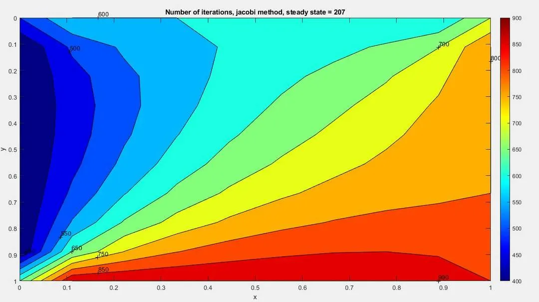

Gauss seidel method

function T_gauss = gauss_method(x,y,dx,dy,nx,ny,T,T_old,error,tolerance,k,solver_type)

gauss_iter = 0;
while(error>tolerance)
    for i = 2:nx-1
        for j = 2:ny-1
            
           term1 = (T(i-1,j) + T_old(i+1,j))/(dx^2);
           term2 = (T(i,j-1) + T_old(i,j+1))/(dy^2);
           T(i,j) = (1/k)*(term1+term2);
        end
    end
    error = max(max(abs(T_old-T)));
    T_old = T;
    gauss_iter = gauss_iter + 1;
   
end
figure(solver_type)
T_gauss = T;
contourf(x,y,T)
colormap(jet);
title_heading = sprintf('Number of iterations, gauss seidel method, steady state = %d', gauss_iter);
title(title_heading)
xlabel('x')
ylabel('y')
colorbar
set(gca,'ydir','reverse')
pause(0.03)

end'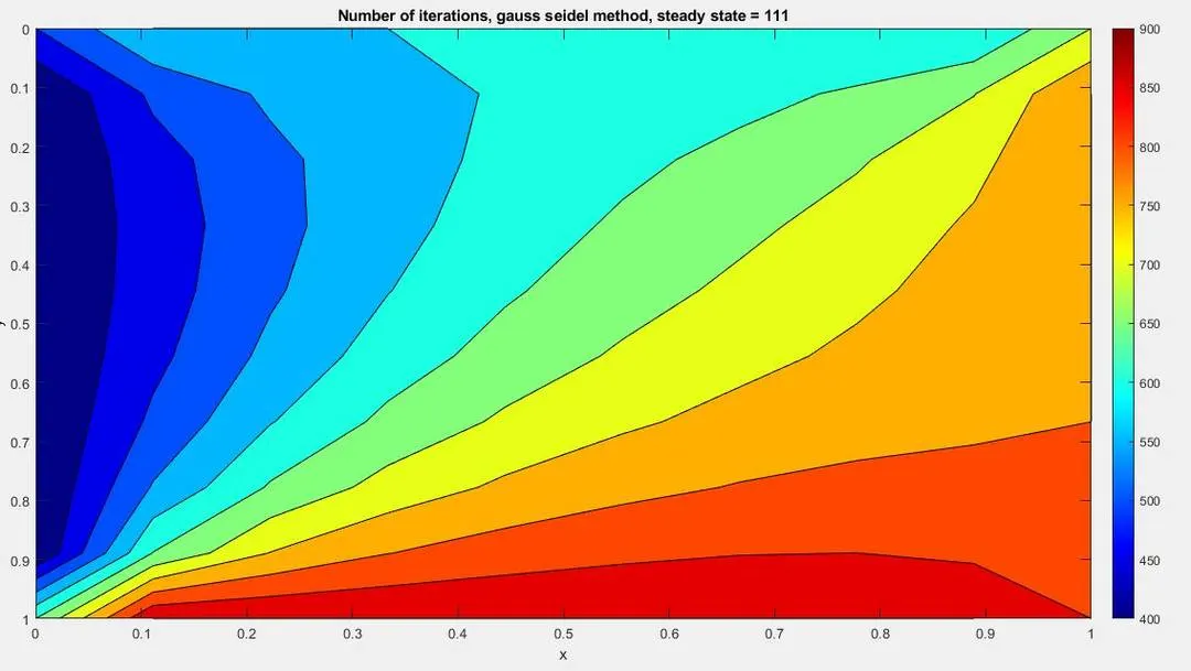

Succesive over relaxation method

function T_sor = sor_method(x,y,dx,dy,nx,ny,T,T_old,error,tolerance,k,solver_type)

omega = 1.1;
sor_iter = 0;
while(error>tolerance)
    for i = 2:nx-1
        for j = 2:ny-1
            
           term1 = (T(i-1,j) + T_old(i+1,j))/(dx^2);
           term2 = (T(i,j-1) + T_old(i,j+1))/(dy^2);
           T(i,j) = ((1-omega)*T_old(i,j)) + ((omega/k)*(term1+term2));
        end
    end
    error = max(max(abs(T_old-T)));
    T_old = T;
    sor_iter = sor_iter + 1;
    

end
 figure(solver_type)
T_sor = T;
contourf(x,y,T)
colormap(jet);
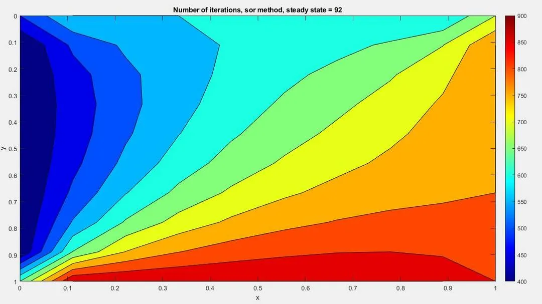
title_heading = sprintf('Number of iterations, sor method, steady state = %d', sor_iter);
title(title_heading)
xlabel('x')
ylabel('y')
colorbar
set(gca,'ydir','reverse')
pause(0.03)

end

Step 4- Solving the transient state 2D conduction equation using an explicit scheme

The transient equation,

`(delT)/(delt) + alpha((del^2T)/(delx^2) + (del^2T)/(dely^2) ) = 0`

This can be written as

And the function:

function T_transient_explicit = transient_explicit(x,y,nt,nx,ny,T,T_old,tolerance,k1,k2,cfl)

no_of_iter = 0;
for k = 1:nt
error = 9e9;
while(error>tolerance)
    for i = 2:nx-1
        for j = 2:ny-1
           term0 = T_old(i,j);
           term1 = k1*((T_old(i+1,j)) - (2*T_old(i,j)) + (T_old(i-1,j)));
           term2 = k2*((T_old(i,j+1)) - (2*T_old(i,j)) + (T_old(i,j-1)));
           T(i,j) = term0 + term1 + term2;
        end
    end
    error = max(max(abs(T_old-T)));
    T_old = T;
    no_of_iter = no_of_iter+1;


end


end

T_transient_explicit = T;
contourf(x,y,T)
clabel(contourf(x,y,T))
colormap(jet);
title_heading = sprintf('Number of iterations, explicit, transient state = %d, cfl = %d', no_of_iter,cfl);
title(title_heading)
xlabel('x')
ylabel('y')
colorbar
set(gca,'ydir','reverse')




end

However, running the code with a large timestep size, dt = 300 and number of timesteps 1400 in this case leads to an error as the CFL courant number criterion of 1 is not met.

This results in a wrong output as seen below

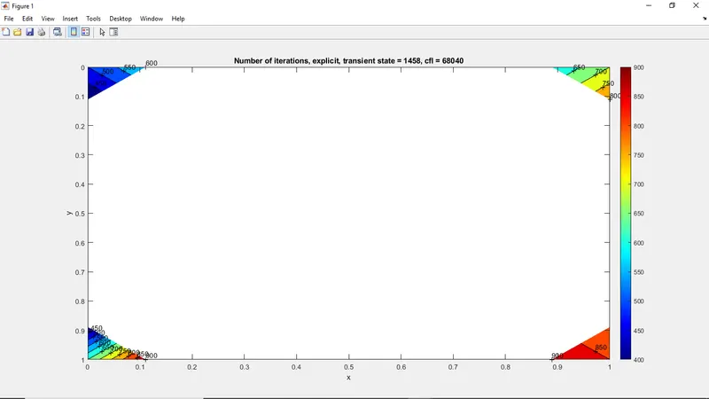
Clearly, the courant number is too high and thus the timestep size must be reduced drastically, to say, 1e-3 in this case.

Then, a correct expected output can be seen below

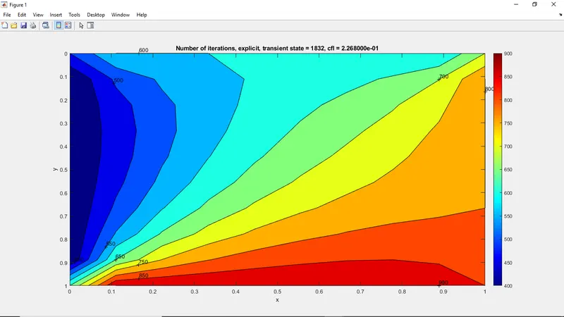
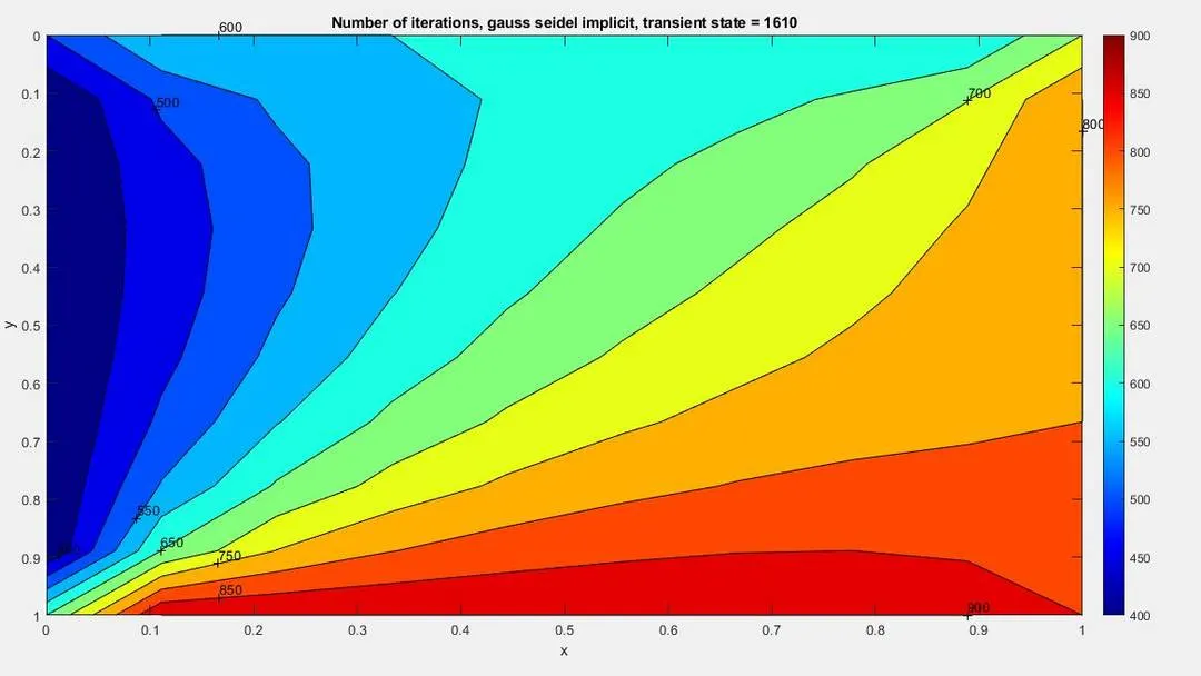
To avoid this issue relating to the timestep size, an implicit scheme can be used with a timestep size of any number as it is unconditionally stable and independent of the time step size.

Three iterative solvers are used for the implicit schemes:

Jacobi

function jacobi_trans_state = jacobi_transient(x,y,nx,ny,nt,T,T_old,tolerance,k1,k2)
no_of_iter = 1;
T_previous = T;

for k = 1:nt
    error = 9e9;
    while (error>tolerance)
    
        for i = 2:nx-1
            for j = 2:ny-1
                term_1  = ((1 + (2*k1) + (2*k2)))^-1;
                term_2 = k1*term_1;
                term_3 = k2*term_1;
                H = (T_old(i-1,j)) + (T_old(i+1,j));
                V = (T_old(i,j+1)) + (T_old(i,j-1));
                T(i,j) = (T_previous(i,j)*term_1) + (H*term_2) + (V*term_3);
            end
        end
    error = max(max(abs(T_old-T)));
    T_old = T;
    no_of_iter = no_of_iter + 1;
    

       
    end
    T_previous = T;
 
  
end


jacobi_trans_state = T;
contourf(x,y,T)
clabel(contourf(x,y,T))
colormap(jet);
title_heading = sprintf('Number of iterations, jacobi implicit, transient state = %d', no_of_iter);
title(title_heading)
xlabel('x')
ylabel('y')
colorbar
set(gca,'ydir','reverse')



end

Gauss seidel

function gauss_trans_state = gauss_transient(x,y,nx,ny,nt,T,T_old,tolerance,k1,k2)
no_of_iter = 1;
T_previous = T;

for k = 1:nt
    error = 9e9;
    
    while (error>tolerance)
        for i = 2:nx-1
            for j = 2:ny-1
                term_1  = ((1 + (2*k1) + (2*k2)))^-1;
                term_2 = k1*term_1;
                term_3 = k2*term_1;
                H = (T(i-1,j)) + (T_old(i+1,j));
                V = (T(i,j+1)) + (T_old(i,j-1));
                T(i,j) = (T_previous(i,j)*term_1) + (H*term_2) + (V*term_3);
            end
        end
    error = max(max(abs(T_old-T)));
    T_old = T;
    no_of_iter = no_of_iter + 1;
    

       
    end
    T_previous = T;
 
    

end

figure(1)
gauss_trans_state = T;
contourf(x,y,T)
clabel(contourf(x,y,T))
colormap(jet);
title_heading = sprintf('Number of iterations, gauss seidel implicit, transient state = %d', no_of_iter);
title(title_heading)
xlabel('x')
ylabel('y')
colorbar
set(gca,'ydir','reverse')


end

Succesive over relaxation

function sor_trans_state = sor_transient(x,y,nx,ny,nt,T,T_old,tolerance,k1,k2)
no_of_iter = 1;
T_previous = T;
T_end = T;
omega = 1.3;
for k = 1:nt
    error = 9e9;
    while (error>tolerance)
        for i = 2:nx-1
            for j = 2:ny-1
                term_1  = ((1 + (2*k1) + (2*k2)))^-1;
                term_2 = k1*term_1;
                term_3 = k2*term_1;
                H = (T(i-1,j)) + (T_old(i+1,j));
                V = (T(i,j+1)) + (T_old(i,j-1));
                T(i,j) = (T_previous(i,j)*term_1) + (H*term_2) + (V*term_3);
                T_end(i,j) = ((1-omega)*T_old(i,j)) + (T(i,j)*omega);
            end
        end
    error = max(max(abs(T_old-T)));
    T_old = T_end;
    no_of_iter = no_of_iter + 1;
    
    end
    T_previous = T_end;
 
    

end

figure(1)
sor_trans_state = T;
contourf(x,y,T)
clabel(contourf(x,y,T))
colormap(jet);
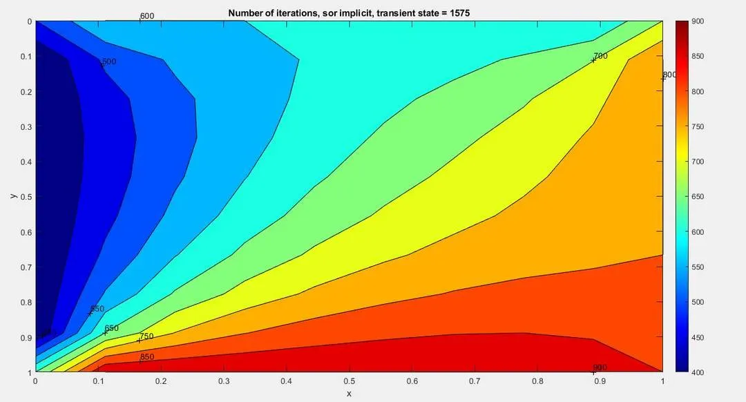
title_heading = sprintf('Number of iterations, sor implicit, transient state = %d', no_of_iter);
title(title_heading)
xlabel('x')
ylabel('y')
colorbar
set(gca,'ydir','reverse')


end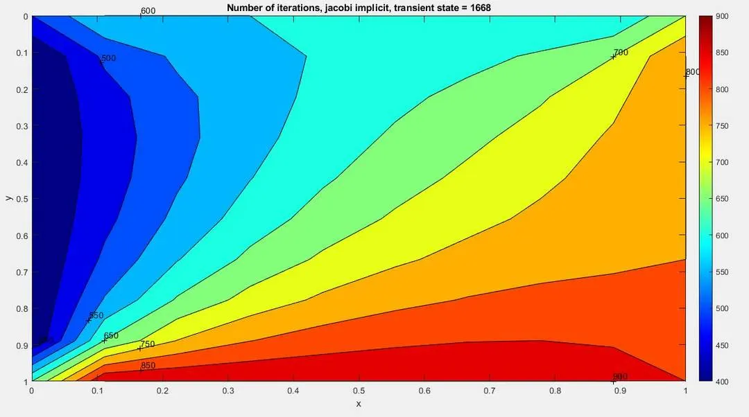

Inferences

The steady state condition can easily be solved using iterative solvers as there is no time derivative involved.

However, in order to solve the transient state equation, two schemes can be used, explicit or implicit.

While the explicit scheme is much easier to understand and is simpler, it has a courant number limitation where the timestep size must be small enough such that the courant number should not exceed one.

To solve this limitation, an implicit scheme using an iterative solver can be used as an implicit finite-difference approximation is unconditionally stable, that is, independent of the timestep size.

Coming to the tyes of iterative solvers used, Succesive over relaxation method could be the best choice to acheive convergence as it takes a lesser number of iterations to attain steady state.