Week 5 - Literature review: ODE Stability
Stability of an Ordinary Differential Equation:
In Reacting flows, rate of change of molar concentration of each species has to be determined. The concentration of each species is expressed in the form of coupled non linear ordinary differential equations of all other species. These ODEs need to be solved to get the molar concentrations. These can be solved by two methods : explicit and implicit.
Lets consider an ODE `dy/dt = -10000*y - e^(-t)` ---> (1`
where 'y' can be molar concentration of any species in the reaction mechanism
'dy/dt' would be the rate of change of molar concentration of that species.
As this involves time, time marching technique is used. Molar concentration after a particular time can be found out.
The molar concentrations at time t=0 are given and values at next time steps are calculated.
Two approaches can be used to solve the above ODE.
1. Explicit approach:
In this, the RHS of the ODE has all known values i.e, values of previous time steps. The values at LHS has to be found.
Discretizing eq. (1),
`(y^(n+1) - y^n)/dt = -10000*y^n - e^(-t)`
where `y^n` is the value of y at time step 'n'.
`y^(n+1)`is the value of y at next time step 'n+1'
Rearranging,
`y^(n+1) = y^n - 10000y^n*dt - e^(-t)*dt` ---> (2)
In the above eq., values of y at RHS are all known. There is only one unknown variable. Substituting the known values gives the unknown at LHS.
2. Implicit approach:
In this, the RHS of the ODE contains unknown values i.e., values of variables at next time step.
Discretizing eq. (1) using backward difference method,
`(y^(n) - y^(n-1))/dt = -10000*y^n - e^(-t)`
Rearranging,
`y^n = (y^(n-1) - e^(-t)dt)/(1+10000dt)` ---> (3)
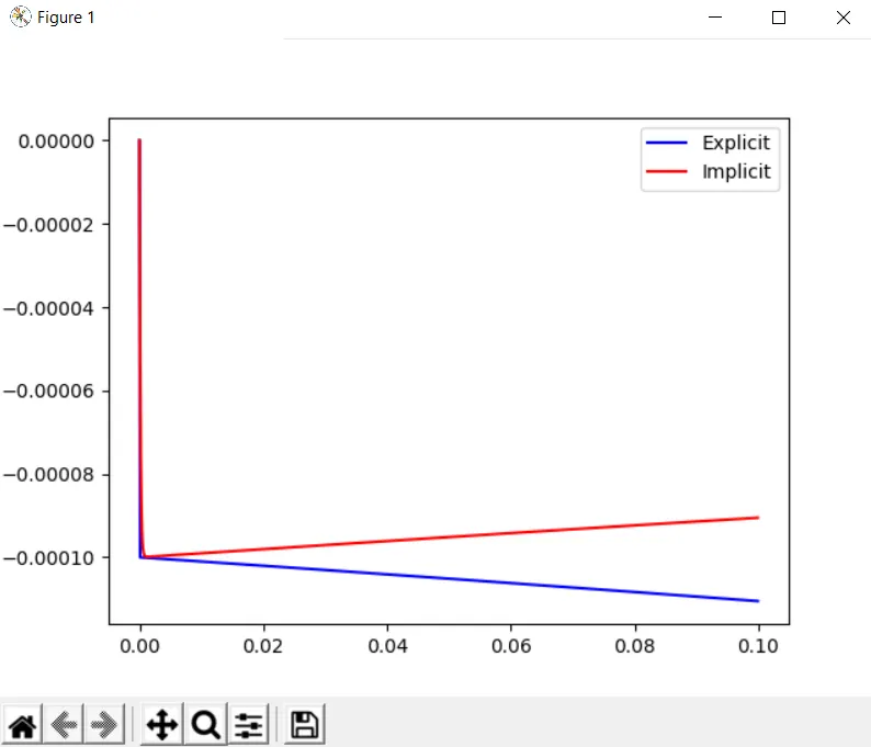
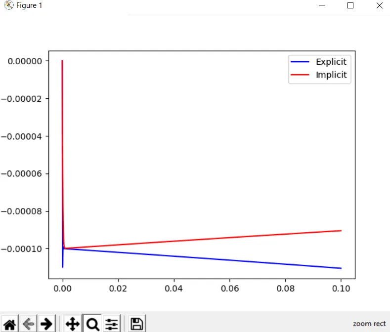
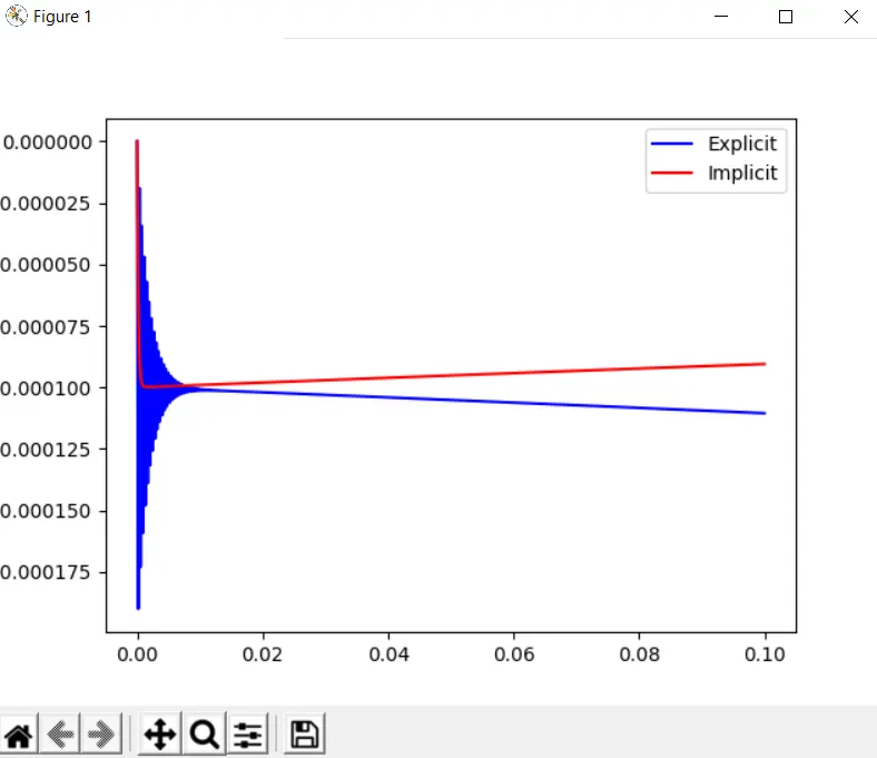
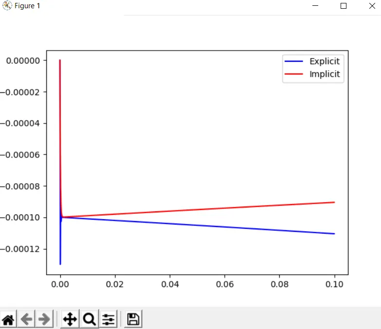
Codes in python are written to solve the ODE in both explicit and implicit approach and check which approach would give more accurate results. The trend for different values of 't' is obtained. Time step size is varied randomly each time.
At dt = 0.0002:
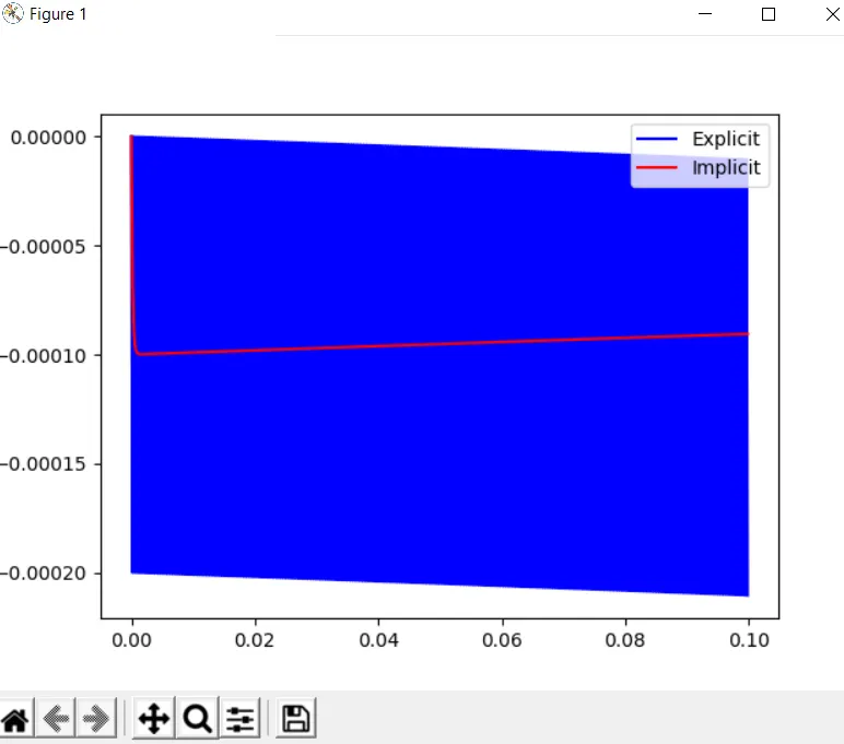
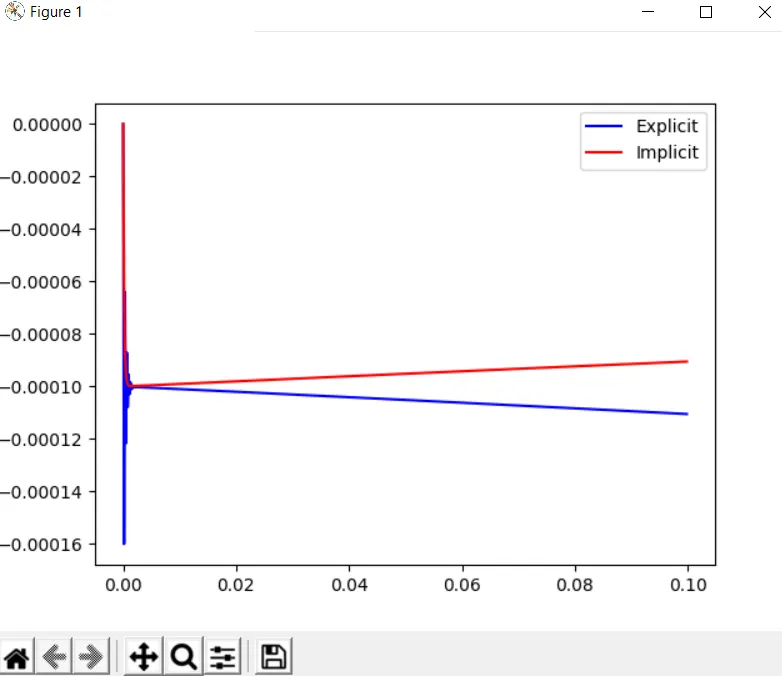
The above plots are obtained for various time step sizes. It can be observed that explicit approach approach does not always give a stable solution whereas the impliit approach gives stable solution irrespecive of time step size. It can be inferred that the stability of solution of an ODE is depending on the independent variable (dt).
Here, it can be seen that the implicit approach does not depend on time step size. It always gives stable results. Also, time step size can be large so the solution converges quickly. But if a system has a no. of ODEs, it becomes difficult to solve using implicit approach. The code becomes very long and complex.
The solution becomes unstable if the error increases with every time step. So, it can be said that the explicit approach is conditionally stable i.e., it gives stable solution only within a limiting value of dt. This is called the stability criterion. Each ODE has a particular stability condition. If the ODE violates the stability condition, result would be unstable. In the above case, stability depends on time step size (dt). As seen above, in every other case except the first one, ODE might not be satisfying the stability condition and hence the result has wiggles. But the advantage of explicit approach is its easy to solve as the code will be relatively simple.
So, it would be beneficial to use explicit approach if used within a particular limit called the stability condition.
If the approach used does not provide stable results, it would be impossible to find the behaviour of governing equation and thereby flow properties at various locations and times cannot be obtained. That is why stability of a solution is of utmost importance.
Stability condition for every ODE should be derived and the value of independent variable should be less than limit set by stability criterion.
Deriving stability condiion for eq. (1):
As mentioned before, solution becomes unstable if the error increases with time.
Therefore, for a solution to be stable,
`mod(epsilon^(n+1)/epsilon^n) <= 1` ---> (4)
where `epsilon` is the error.
The error always satisfies the governing equation.
Therefore, in explicit approach equation,
`(epsilon^(n+1) - epsilon^n)/dt = -10000*epsilon^n - e^(-t)` ---> (5)
Also, error can be expressed as `e^(at)*e^(ik_my)` ---> (6)
Substituitng (6) in (4),
`mod(epsilon^(n+1)/epsilon^n) = mod(e^(adt)) <= 1` ---> (7`
Substituting (6) in (5),
`(e^(a(t+dt))*e^(ik_my) - e^(at)*e^(ik_my))/dt = -10000*(e^(at)*e^(ik_my)) - e^-t`
Rearranging,
`(e^(at).e^(ik_my)*(e^(adt)-1))/dt = -10000*(e^(at)*e^(ik_my)) - e^(-t)`
`(e^(adt) - 1)/dt = -10000 - (e^-t/(e^(at)*e^(ik_my)))`
`e^(adt) - 1= -1000*dt - (e^-t*e^(-at)*e^(-ik_my)*dt)`
`e^(adt) = 1 - (10000 + e^-(t+at)*e^(-ik_my))*dt`---> (8)
Substituting (8) in (7),
`mod(1 - (10000 + e^-(t+at)*e^(-ik_my))*dt) <= 1`
Two conditions are possible,
1. `1 - (10000 + e^-(t+at)*e^(-ik_my))*dt <= 1`
`(10000 + e^-(t+at)*e^(-ik_my))*dt>= 0`
dt cannot be negative. So it can be inferred that
`(10000 + e^-(t+at)*e^(-ik_my))` should always be positive but this condition does not set a limit on the dt value.
2. `1 - (10000 + e^-(t+at)*e^(-ik_my))*dt >= -1`
`(10000 + e^-(t+at)*e^(-ik_my))*dt -1 <= 1`
let `e^(-(t+at))*e^(-ik_my) = K`
`(10000 + K)dt <= 2`
`dt <= 2/(10000 + K)`
K is the exponential function to the power of negative numbers and are very small compared to 10000 and can be neglected.
So, `dt <= 0.0002`
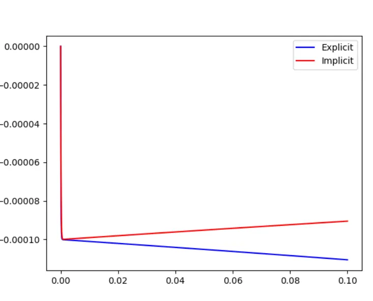
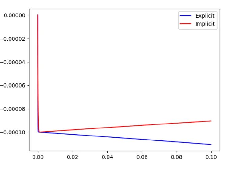
So, to obtain a stable solution (or) in order for the solution to be of some meaning, the time step size should be less than 0.0002. (when using an explicit approach)
From the plots shown above, for a value of dt = 0.0002, it can be seen that the solution has so many wiggles and atleast does not give an idea of what the behavior of the ODE would be.
Plots with time step size less than 0.0002:
For dt = 0.00003:
For dt = 0.00008:
For dt = 0.0001:
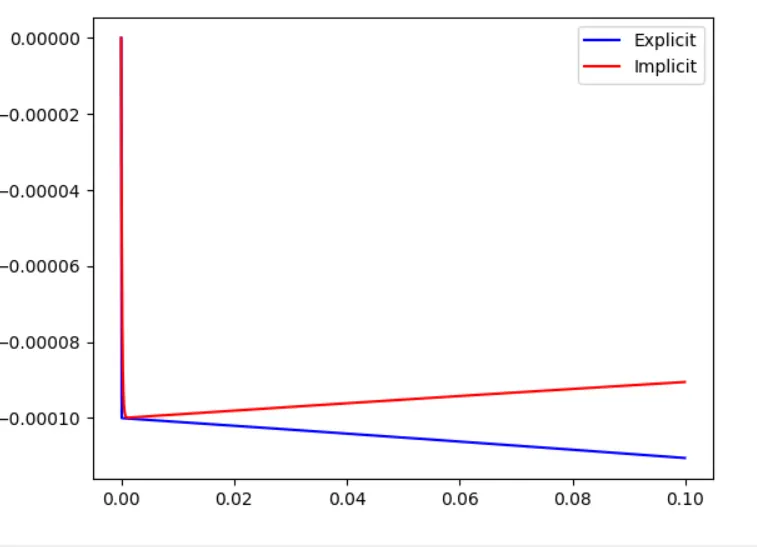
As observed from above plots, when the time step size is less than 0.0002, explicit approach gives stable solution.
Google drive link for code:
https://drive.google.com/drive/folders/1G8aWuKKxrX8xjiT06gboZl61m3zvsV0d