Week 5 - Genetic Algorithm

Aim:

To create MATLAB code for a Genetic Algorithm to optimise the Stalagmite function and identify the function's global maxima.

Objective:

The purpose of this report is to demonstrate the concept of genetic algorithms and the syntax of "ga" in MATLAB while optimising the stalagmite function through programming in MATLAB using a genetic algorithm.

Theory:

The natural evolution theory of Charles Darwin serves as the foundation for the search heuristic known as a genetic algorithm. The fittest people are chosen to reproduce in order to give rise to the following generation of offspring, as is the case in natural selection, which is what our algorithm reflects.

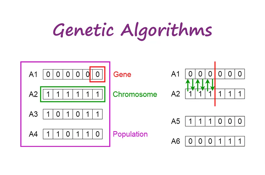
Phases in Genetic Algoritham-

1. Initialization of Population (Coding)

The code generates its random population of defined size and from that population the code evaluates the fitness of the members of the population according to which it forms new population based on no. of iterations performed.

A.Fitness Function

It is that function which we have to optimize and its optimization is done with the help of number of generations which have been formed by the code accordance with the fitness value of each member generated, these fitness values are used for the reproduction of the children.

Selection

The idea of the selection phase is to select the fittest individuals and let them pass their genes to the next generation. The main goal of this phase is to find the region where the chances of getting the best solution are more.

Inspiration for this is from the survival of the fittest.

It should be a balance between exploration and exploitation of search space.

GA tries to move the genotype to higher fitness in the search space.

Too strong fitness selection bias can lead to sub-optimal solutions.

Too little fitness bias selection results in unfocused search.

Reproduction

Generation of offspring happen in 2 way:

a. Crossover

b. Mutation

a) Crossover

Crossover is the most significant stage in the genetic algorithm. During crossover, a random point is selected while mating a pair of parents to generate offspring.

There are 3 major types of crossover.

Single Point Crossover:

A point on both parents’ chromosomes is picked randomly, and designated a ‘crossover point’.

Two-Point Crossover: Two crossover points are picked randomly from the parent chromosomes.

Unifofm Crossover: In a uniform crossover, typically, each bit is chosen from either parent with equal probability.

b) Mutation

In a few new offspring formed, some of their genes can be subjected to a mutation with a low random probability. This indicates that some of the bits in the bit chromosome can be flipped. Mutation happens to take care of diversity among the population and stop premature convergence.

Function calling code:

function [f] = stalagmite(input_value)

f1x = (sin(5.1*pi*input_value(1) + 0.5)).^6;

f1y = (sin(5.1*pi*input_value(2) + 0.5)).^6;

f2x = exp(-4*log(2)*(((input_value(1) - 0.0667).^2)/(0.64)));

f2y = exp(-4*log(2)*(((input_value(2) - 0.0667).^2)/(0.64)));

f = -(f1x*f1y*f2x*f2y);

end

Program code:

Study 1:

clear all 
close all
clc

x = linspace(0,0.6,150);
y = linspace(0,0.6,150);
num_cases = 50;

% creating a 2D mesh
[xx,yy] = meshgrid(x,y);

%Evaluating Stalagmite function
for i = 1:length(xx)
    for j = 1:length(yy)
        input_value(1)=xx(i,j);
        input_value(2)=yy(i,j);
        f(i,j) = stalagmite(input_value);
    end
end

% Study1- Unbounded statistical behaviour
tic
for i = 1:num_cases
    [inputs1, fopt1(i)] = ga(@stalagmite, 2);
    xopt(i) = inputs1(1);
    yopt(i) = inputs1(2);
end
study1_time = toc;

figure(1)
subplot(2,1,1)
hold on
surfc(xx,yy,-f)
xlabel('X-Values')
ylabel('Y-Values')
zlabel('Function Values')
shading interp
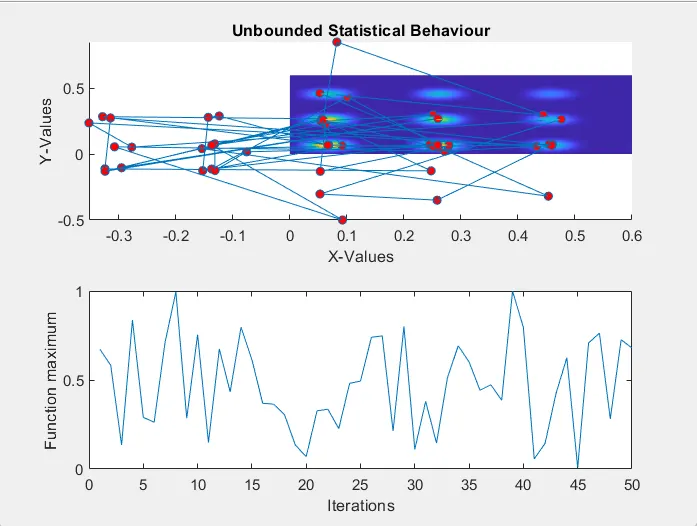
plot3(xopt,yopt,-fopt1,'marker','o','markersize',5,'markerfacecolor','r')
title('Unbounded Statistical Behaviour')
subplot(2,1,2)
plot(-fopt1)
xlabel('Iterations')
ylabel('Function maximum')

Output 1:

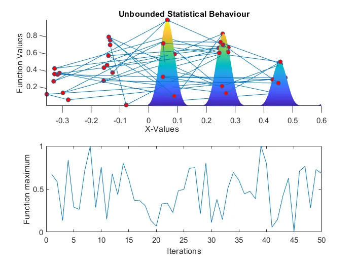
Unbounded Statistical Behaviour Plot :- (Iterations = 50)

Study 2:

% Study2 - Statistical behaviour with upper aned lower bound
tic
for i = 1:num_cases
    [inputs2,fopt2(i)] = ga(@stalagmite,2,[],[],[],[],[0;0],[1;1]);
    xopt(i) = inputs2(1);
    yopt(i) = inputs2(2);
end
study2_time = toc

figure(2)
subplot(2,1,1)
hold on
surfc(xx,yy,-f)
xlabel('X-Values')
ylabel('Y-Values')
zlabel('Function Values')
shading interp
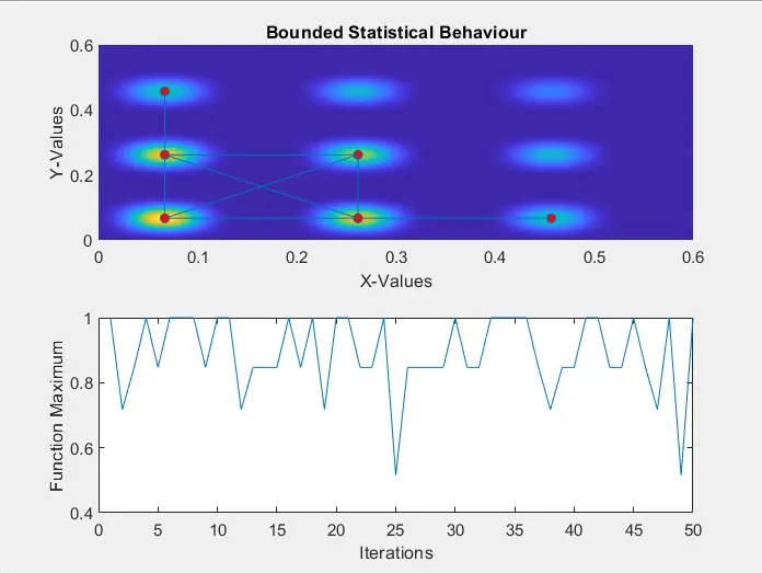
plot3(xopt,yopt,-fopt2,'marker','o','markersize',5,'markerfacecolor','r')
title('Bounded Statistical Behaviour')
subplot(2,1,2)
plot(-fopt2)
xlabel('Iterations')
ylabel('Function Maximum')

Output 2:

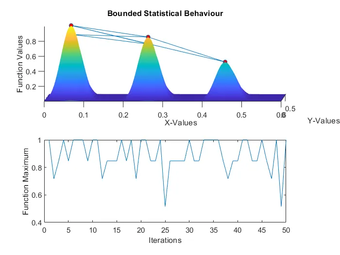
Bounded Statistical Behaviour Plot :- (Iterations = 100)

Study 3:

%Study3- increasing GA iterations (Population size)
options = optimoptions('ga');
options = optimoptions(options,'PopulationSize',170);

tic
for i = 1:num_cases
    [inputs3, fopt3(i)] = ga(@stalagmite,2,[],[],[],[],[0;0],[1;1],[],[],options);
    xopt(i) = inputs3(1);
    yopt(i) = inputs3(2);
end
study3_time = toc

figure(3)
subplot(2,1,1)
hold on
surfc(xx,yy,-f)
xlabel('X-Values')
ylabel('Y-Values')
zlabel('Function Values')
shading interp
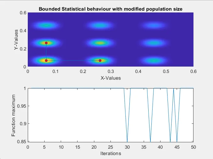
plot3(xopt,yopt,-fopt3,'marker','o','markersize',5,'markerfacecolor','r')
title('Bounded Statistical behaviour with modified population size')
subplot(2,1,2)
plot(-fopt3)
xlabel('Iterations')
ylabel('Function maximum')

Output 3:

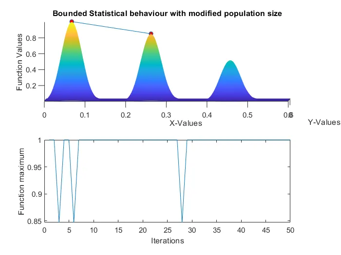
Modified Population Size Plot :- (Iterations = 170)

Total_time = study1_time + study2_time + study3_time
fprintf('n The results are below : ')

fprintf('nn study 1 : Unbounded statistical Bahaviour')
fprintf('nn The time taken for the study-1 is : %f',study1_time)
fprintf('n The co-ordinates of x & y for the global Maxima of the function are : %f,%f',inputs1(1),inputs1(2))
fprintf('nn the global maxima of the  function is : %f',-(mean(fopt1)))

fprintf('nn study 2 : Unbounded statistical Bahaviour')
fprintf('nn The time taken for the study-2 is : %f',study2_time)
fprintf('n The co-ordinates of x & y for the global Maxima of the function are : %f,%f',inputs2(1),inputs2(2))
fprintf('nn the global maxima of the  function is : %f',-(mean(fopt2)))

fprintf('nn study 3 : Unbounded statistical Bahaviour')
fprintf('nn The time taken for the study-3 is : %f',study3_time)
fprintf('n The co-ordinates of x & y for the global Maxima of the function are : %f,%f',inputs3(1),inputs3(2))
fprintf('nn the global maxima of the  function is : %f',-(mean(fopt3)))

Explantion:

1. First, the Linspace command is used to define x & y with 150 elements between zero and 0.6 including the bounds.
2. Then num_cases is set which will be used as counter for iteration to 50
3. Then a 2D grid is made using meshgrid command is created from x & y input tobe output to xx & yy
4. Then for loop is used to solve the genetic algorithm for every element in the 2D mesh grid
5. The length of rows & column (which have equal length) are used as counters
6. Then the input vector is declared as ga requires input vector which is each value in the mesh grid
7. Then output of stalagmite function is stored in matrix
8. Then tic command is used to start a timer
9. Then for loop bounded by the number of iterations is formed
10. Then smallest (minimum) value of the function for each iteration is output & its x & y coordinates which are stored in separate variables.
11. Then 'toc' command is used to stop the timer and the output is stored in study_time1
12. Then figure1 is plotted by the following steps-
13. First subplot command is used to partition the plot window in order to draw more than one plot in the same window, two rows and one column are specified and then the position of each plot is selected
14. Then hold on command is used to prevent plot for being removed
15. The surfc command is used to plot contour with xx & yy value from the mesh grid as input and negative optimum value is used because we need to maximize the function
16. Then x,y,& z axis are labelled
17. Then shading interp is used to smoothen the function plot and to remove the grid lines
18. Then plot 3 command is used to plot a point in 3D, here it will plot- fopt because we need the maximum value of the function not the minimum
19. Then the graph title is selected

Outputs:

Errors:

1. Mention distinct input vector sizes, x and y, while defining the inputs. The mesh grid instruction is primarily to blame for the problem, as the two vectors' different diameters prevent them from being joined.

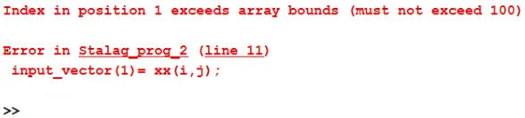
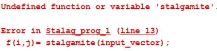
2. Undefined function or variable

Results:

1. Unbounded statistical Behaviour-

The time taken for the study-1 = 5.912489 sec

The global maxima of the function = 0.512086

2. Bounded statistical behaviour-

Time taken for the study-2 = 7. 937613 sec

The global maxima of the function = 0.905461

3. Bounded statistical behaviour with increase population size -

Time taken for the study-3 = 19.544688 sec

The global maxima of the function = 0.993887

The total time taken to complete the total study = 33.305790.