Week 4.1 - Solving second order ODEs

Aim:

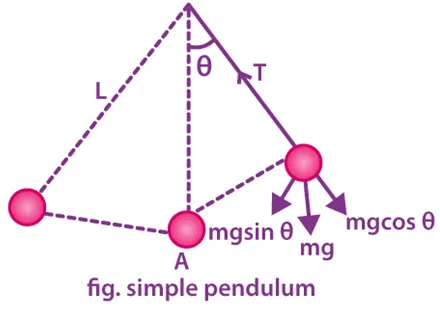
The aim of the challenge is to write a program that solves the following ODE and this ODE represents the equation of motion of a simple pendulum with damping.

Objective:

The objective of the challenge is to write a report that consist of step wise explanation of your code, errors faced while programming, the steps to overcome those errors and good presentaion of the code with line by line explanation.

• Using the built-in MATLAB function for solving ordinary differential equations to create the function.
• To create a simple pendulum animation.

Important terms:

• The oscillatory motion of a simple pendulum: Oscillatory motion is defined as the to and fro motion of the pendulum in a periodic fashion and the centre point of oscillation known as equilibrium position.
• The time period of a simple pendulum: It is defined as the time taken by the pendulum to finish one full oscillation and is denoted by “T”.
• The amplitude of simple pendulum: It is defined as the distance travelled by the pendulum from the equilibrium position to one side.
• Length of a simple pendulum: It is defined as the distance between the point of suspension to the centre of the bob and is denoted by “l”.

Program code:

1. Main code

close all
clear all
clc

% inputs
b = 0.05;
m = 1;
L = 1;
g = 9.81;

%time spans
t_span = linspace(0,20,500);

 % [angle displacement,velocity]
theta_0 = [0;3];

%ode solver
[t,results] = ode45(@(t,theta) ode_function(t,theta,b,g,m,L),t_span,theta_0);

figure(1)
%plot all rows from first column
plot(t,results(:,1));

% hold on used to get all the data from the plot.
hold on

%plot all rows from second column
plot(t,results(:,2));

% providing title, x and y-axis to the plot
grid on
title('Displacement vs Time');
xlabel('Time');
ylabel('Plot');

ct = 1;
theta1 = results(:,1); %all rows from first column which are angle values
for i = 1:length(theta1)
    % creating x0 and y0.
    x0 = 0; 
    y0 = 0;
    theta2 = theta1(i);
    % creating x1 and y1 
    x1 = 1*sin(theta2);
    y1 = -1*cos(theta2);
    figure(2)
    plot([-1 1],[0,0],'linewidth',3,'color','r'); % hinge to the stick the pendulum
    hold on
    plot([0,0],[-2 2],'--',[x0 x1][y0,y1],'o','MarkerSize',10,'MarkerFaceColor','b','MarkerEdgeColor','g','linewidth',6); % %plotting lines from hinge to the end with a ball marker at the end
    hold on
    axis([-2 2 -2 2]) % creating axis to the plot
    line([x0 x1],[y0 y1],'linewidth',2) % line act line a thread to move with the balls
    hold off
    title('Simple pendulum animation')
    M(ct)=getframe(gcf);       
    ct=ct+1; 
end
movie(M) %starting to create a video file
Videofile=VideoWriter('pendulum.avi','Uncompressed AVI');  %creating a video file named pendulum with avi extension
open(Videofile) %open the video file
writeVideo(Videofile,M) %write the plot images to the fideo file
close(Videofile)  %close the video file. 

2. Function code:

function [dtheta_dt] = ode_function(t,theta,b,g,m,L)
theta1 = theta(1);
theta2 = theta(2);
dtheta1_dt = theta2;
dtheta2_dt = -(b/m)*theta2 - (g/L)*sin(theta1);
dtheta_dt = [dtheta1_dt;dtheta2_dt];
end

Explanation:

1. First off all I described all input values which are required pendulum settings.

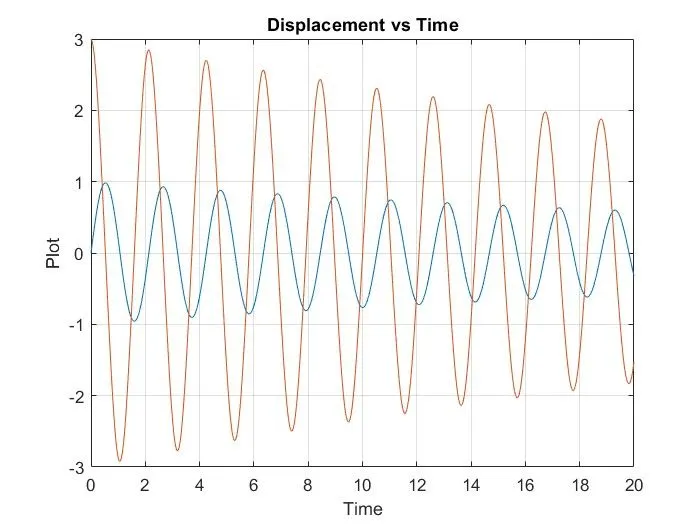
2. Then simulate the motion between 0-20 sec, for angular displacement = 0, angular velocity = 3 rad/sec at time t = 0.

3. Then solve the ODE by using 'ode45' function, in which I describe time & theta.

4. Then plot the some figures

5. In first figure angular displacement start from 0 sec while angular velocity starts from 3 rad/sec, and graph showing sine wave and it decreases slightly from start to end.

6. In second figure used for loop to showing all the movement from left to right directions.

7. The hinge to stick the pendulum starts from [-1 1] and [0 0].

8. Then the ball start form the [x0 x1] and [y0 y1]. The markersize, markerfacecolor and markeredgecolor is given to the bob ro oscillate.

9. Creating axis and the thread using line to the pendulum to oscillate.

10.For plotting all frames in movie file I use getframe command.

11. Creating movie, videofile by saving in the extension of .avi which is uncompressed file.

12. Open video file edited and close it again as shown in MATLAB code.

13. In function file, describe all the important function values.

14. It's the solution of pendulum equation where mentioned theta1, theta2 to solve the ODE equation.

Output:

1. The angular diplacement and angular velocity with respect to time,

2. Pendulum animation:

The output is in an animated video clip. The youtube link is attached below.

https://youtu.be/z82YatRsEhk

3. Error and solution

• There are many errors that occurs while generating g loop for animation.
• The main cause of the error I faced is a typo which was \" results(i:1)\" which is not correct.
• The correct form for this program is \"results(i,1)\".
• I faced many more errors because typo\'s in creating animation in octave.

Conclusion:

The program to solve the ODEs and simple pendulum animation is successfully done using MATLAB.