Week 5 - Genetic Algorithm
Introduction to Optimization:
Optimization is the process of making something better. In any process, we have a set of inputs and a set of outputs as shown in the following figure.
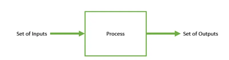
Optimization refers to finding the values of inputs in such a way that we get the “best” output values. The definition of “best” varies from problem to problem, but in mathematical terms, it refers to maximizing or minimizing one or more objective functions, by varying the input parameters.
The set of all possible solutions or values which the inputs can take make up the search space. In this search space, lies a point or a set of points that gives the optimal solution. The aim of optimization is to find that point or set of points in the search space.
THE GENETIC ALGORITHM:
Nature has always been a great source of inspiration to all mankind. Genetic Algorithms (GAs) are search-based algorithms based on the concepts of natural selection and genetics. GAs are a subset of a much larger branch of computation known as Evolutionary Computation.
In GAs, we have a pool or a population of possible solutions to the given problem. These solutions then undergo recombination and mutation (like in natural genetics), producing new children, and the process is repeated over various generations. Each individual (or candidate solution) is assigned a fitness value (based on its objective function value) and the fitter individuals are given a higher chance to mate and yield more “fitter” individuals. This is in line with the Darwinian Theory of “Survival of the Fittest”.
In this way, we keep “evolving” better individuals or solutions over generations, till we reach a stopping criterion.
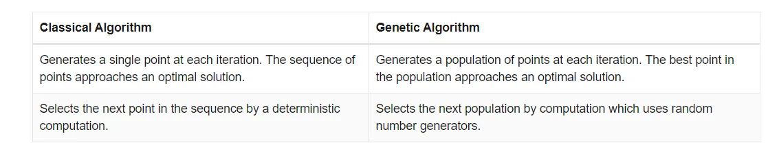
Genetic Algorithms are sufficiently randomized in nature, but they perform much better than random local search (in which we just try various random solutions, keeping track of the best so far), as they exploit historical information as well.
Advantages of GAs
GAs have various advantages which have made them immensely popular. These include −
-
Does not require any derivative information (which may not be available for many real-world problems).
-
Is faster and more efficient compared to the traditional methods.
-
Has very good parallel capabilities.
-
Optimizes both continuous and discrete functions and also multi-objective problems.
-
Provides a list of “good” solutions and not just a single solution.
-
Always gets an answer to the problem, which gets better over time.
-
Useful when the search space is very large and there are a large number of parameters involved.
Limitations of GAs
Like any technique, GAs also suffer from a few limitations. These include −
-
GAs are not suited for all problems, especially problems that are simple and for which derivative information is available.
-
The fitness value is calculated repeatedly which might be computationally expensive for some problems.
-
Being stochastic, there are no guarantees of the optimality or the quality of the solution.
-
If not implemented properly, the GA may not converge to the optimal solution.
In this section, we list some of the areas in which Genetic Algorithms are frequently used. These are −
-
Optimization − Genetic Algorithms are most commonly used in optimization problems wherein we have to maximize or minimize a given objective function value under a given set of constraints. The approach to solve Optimization problems has been highlighted throughout the tutorial.
-
Economics − GAs are also used to characterize various economic models like the cobweb model, game theory equilibrium resolution, asset pricing, etc.
-
Scheduling applications − GAs are used to solve various scheduling problems as well, particularly the timetabling problem.
-
Machine Learning − as already discussed, genetics-based machine learning (GBML) is a niche area in machine learning.
-
Robot Trajectory Generation − GAs have been used to plan the path that a robot arm takes by moving from one point to another.
-
Parametric Design of Aircraft − GAs have been used to design aircraft by varying the parameters and evolving better solutions.
-
DNA Analysis − GAs have been used to determine the structure of DNA using spectrometric data about the sample.
-
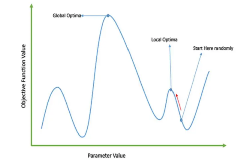
Multimodal Optimization − GAs are obviously very good approaches for multimodal optimization in which we have to find multiple optimum solutions.
-
Traveling salesman problem and its applications − GAs have been used to solve the TSP, which is a well-known combinatorial problem using novel crossover and packing strategies.
-
Neural Networks − GAs are also used to train neural networks, particularly recurrent neural networks.
-
Parallelization − GAs also have very good parallel capabilities, prove to be very effective means of solving certain problems, and also provide a good area for research.
-
Image Processing − GAs are used for various digital image processing (DIP) tasks as well as dense pixel matching.
-
Vehicle routing problems − With multiple soft time windows, multiple depots, and a heterogeneous fleet.
- The stalagmite function is defined separately. This function is later called into the main GA program.
- Now we define the x and y inputs using linspace command.
- Then the input vectors are transformed into an array [xx, yy], so that it can be used to evaluate the functions of two variables and plot three-dimensional mesh/surface plots.
- Now the values in the different matrixes created can be put as input into the function that we have created, by calling it. By this, we can get the value of the stalagmite function at various values of x and y.
- Now since we have got the value of the function at various values, we now need to calculate the maxima value, which can be calculated using the ga command, which is an in-built function in MATLAB.
- Then, the total number of times the ga needs to run is defined using num_cases, and with help of for loop ga is made to run for each iteration and the value is stored in an array.
- GA generally gives the minima value(in built-in MATLAB), but we need the maxima hence we can just inverse the stalagmite function by introducing a 'Negative sign'(This inverses the stalagmite curve, and the Global maxima can be found, instead minima)
- The total study time is calculated using the 'tic' and 'toc' commands at the start and end of the ga for loop respectively.
- The results are then plotted using the surfc command and plot command.
- GA is made to run for 3 iterations, with each iteration having bounded inputs, unbounded inputs, and increasing population size.
Function code for Stalagmite
function [f]= stalagmite(input_vector) %stalagmite function with input as input_vector which contains the x and y variables.
x= input_vector(1);
y= input_vector(2);
f1= (sin(5.1*pi*x+0.5))^6;
f2= (sin(5.1*pi*y+0.5))^6;
f3= exp(-4*log(2)*(x-0.0667)^2/0.64);
f4= exp(-4*log(2)*(y-0.0667)^2/0.64);
f= -(f1*f2*f3*f4); % The Negative sign denotes he inverse of the Stalagmite function and is added in order to find the Maximum value, as GA algorithm always gives the Minimum value.
end
The format for writing genetic algorithms in MATLAB is as follows:

1. x is the local minima point.
2. fun is the function to be called. (In our case, its the stalagmite function)
3. nvars indicates the no of variables used.
4. A and b are used to indicate any kind of inequalities that exist in the function.
5. Aeq and Beq also denote inequalities.
6. lb = lower bound.
7. ub = upper bound.
8. nonlcon gives two vectors representing inequalities and equalities.
9. options are used to perform additional operations like increasing population size. This is done with the help of "optimoptions".
In the first iteration, the behavior of the algorithm is studied by not defining the limits. The GA doesn't run within a particular search space, since we have not defined bounds.
clear all
close all
clc
x=linspace(0,0.6,150); % X value inputs
y= linspace(0,0.6,150);  % Y value inputs
% Even though search space is defined GA Algorithm donot run within this searchspace
[xx,yy]= meshgrid(x,y);

for i = 1:length(xx);
 for j = 1:length(yy);
 input_vector(1)= xx(i,j);
 input_vector(2)= yy(i,j);
 f(i,j)= stalagmite(input_vector);
 end
end

num_cases=50; % GA runs for 50 iterations
tic   % Study Time count start
for i=1:num_cases
 [inputs,f_opt(i)]= ga(@stalagmite,2); % GA function is used to run the stalagmite data and give the optimal solutions.
 x_opt(i)=inputs(1);
 y_opt(i)=inputs(2);
 opt_f(i)= -f_opt(i); %Ga gives us Minima value.Inverse f_opt is taken for Maxima value.

end
study1_time = toc   % Study Time count end

subplot(2,1,1)
hold on
surfc(xx,yy,f) %Generation of stalagmite function.
shading interp  % To bring visually smooth curve surface without mesh lines
plot3(x_opt,y_opt,f_opt,'marker','o','markersize',4,'markerfacecolor','r')%plotting the optimum values with a red dot marker along the stalagmite 3D curves
title('Unbounded inputs')
subplot(2,1,2)
plot(opt_f) %plot of opt_f for every iterations
xlabel('Number of iterations ---->')
ylabel('Function Max -->')
2nd iteration:
Here the lower and upper bounds are defined so as to know the boundaries within which the global maxima lie. In other words, we are defining a definite space within which the global maxima are to be found.
clear all
close all
clc

x=linspace(0,0.6,150);  % X value inputs
y= linspace(0,0.6,150); % Y value inputs
[xx,yy]= meshgrid(x,y);

for i=1:length(xx)
 for j= 1:length(yy)
 input_vector(1)= xx(i,j);
 input_vector(2)= yy(i,j);
 f(i,j)= stalagmite(input_vector);
 %stalagmite function is called for every loop and output is stored in f
 end
end

num_cases=100; % GA runs for 100 iterations
tic         % Study Time start
for i=1:num_cases;
 % Objective function is stalagmite and the number of varaibles is 2
 % A,B,Aeq and Beq = [],as there is no Linear equalities and inequalities constraints in this function
 % lower boundary of varaibles x and y in ga alogorithmn is set as [0,0]
 % upper boundary of varaibles x and y in ga alogorithmn is set as [0.6,0.6]
 [inputs,f_opt(i)]= ga(@stalagmite,2,[],[],[],[],[0,0],[0.6,0.6]);
 x_opt(i)=inputs(1);
 y_opt(i)=inputs(2);
 opt_f(i)= -f_opt(i); %Ga gives us Minima value.Inverse f_opt is taken for Maxima value.
end
study2_time = toc  % Study time end
subplot(2,1,1)
hold on
surfc(xx,yy,f) %Generating the stalagmite function.
shading interp % To bring visually smooth curve surface without mesh lines
plot3(x_opt,y_opt,f_opt,'marker','o','markersize',4,'markerfacecolor','r')
title(' With Bounded inputs')
subplot(2,1,2)
plot(opt_f) %Plotting opt_f value for every iteration
xlabel('Number of iterations ---->')
ylabel('Function Max -->')
3rd iteration:
In this iteration, the population size is increased so as to converge to the Global maxima.
clear all
close all
clc
% x and y inputs
x=linspace(0,0.6,150);
y= linspace(0,0.6,150);
[xx,yy]= meshgrid(x,y);

for i=1:length(xx)
 for j= 1:length(yy)
 input_vector(1)= xx(i,j);
 input_vector(2)= yy(i,j);
 f(i,j)= stalagmite(input_vector);
 end
end

num_cases=150; % GA runs for 150 iterations

options= optimoptions('ga');
options= optimoptions(options,'PopulationSize',450);
tic  % Study Time start
for i=1:num_cases
 % Objective function is stalagmite and the number of varaibles is 2
 % A,B,Aeq and Beq = [],as there is no Linear equalities and inequalities constraints in this function
 % lower boundary of varaibles x and y in ga alogorithmn is set as [0,0]
 % upper boundary of varaibles x and y in ga alogorithmn is set as [0.6,0.6]
 % population size is defined by using options in the algorithmn
 [inputs,f_opt(i)]= ga(@stalagmite,2,[],[],[],[],[0,0],[0.6,0.6],[],options);
 x_opt(i)=inputs(1);
 y_opt(i)=inputs(2);
 opt_f(i)= -f_opt(i); %Ga gives us Minima value.Inverse f_opt is taken for Maxima value.
end

Study3_time = toc   % Study Time end
subplot(2,1,1)
hold on
surfc(xx,yy,f) %Generating the stalagmite function.
shading interp % To bring visually smooth curve surface without mesh lines
plot3(x_opt,y_opt,f_opt,'marker','o','markersize',5,'markerfacecolor','r')
title('Bounded inputs with increased population size')
subplot(2,1,2)
plot(opt_f) %Plotting opt_f value for every iteration
xlabel('Number of iterations ---->')
ylabel('Function Max -->')
ERRORS while programming:
2)
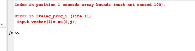
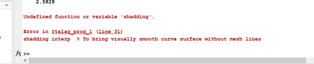
While defining the inputs mentioned different sizes of input vectors x and y. The error is basically due to the mesh grid command where in the two vectors cannot be combined due to their varying sizes.
Apart from this some typos and errors.
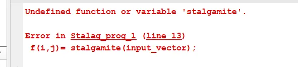
This error was because of not defining the stalagmite.m file before running the code. This was rectified by defining and saving the stalagmite.m function file.
RESULTS & CONCLUSION:
The following are the results obtained on running the GA.
1st iteration: (Iterations = 50)
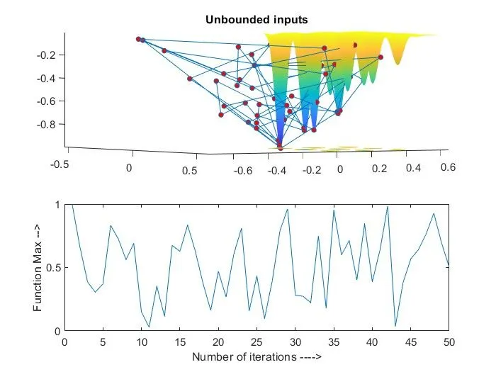
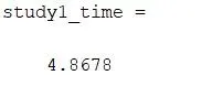
In the above image, it can be seen that since the inputs are boundless GA algorithm has mapped local maxima points outside our stalagmite function. Also, we cannot infer a particular value of global maxima from the above graph, and it is hence pointless.
The study time is very less as the ga algorithm is made only to run for 50 iterations.
2nd Iteration:(iterations = 100)
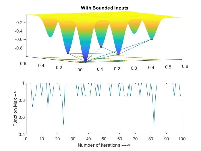

The above graph is more clear and more optimized compared to the 1st iteration since here the bounds were defined and we could get only the values within our range. We are now more clear on the range within which our maxima lie.
3rd Iteration: (iterations = 150)
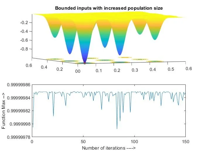
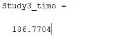
In this case, we are getting the optimized value of global maxima with an accurate range, since we increased the number of iterations and population size.
Since the number of iterations and population size is increased the study time is so high compared to the previous two iterations.
Thus it can be concluded that GA gives more accurate results in the case of bounded inputs and by increasing the number of iterations and population size.
It can also be inferred that even if we define a particular search space for GA, the GA doesn't run inside the search space. Only in cases of bounded inputs we can get interfering able results.
REFERENCES:
- https://www.sciencedirect.com/topics/engineering/genetic-algorithm
- https://en.wikipedia.org/wiki/Genetic_algorithm
- https://in.mathworks.com/help/gads/ga.html
- https://in.mathworks.com/help/gads/genetic-algorithm.html
- https://in.mathworks.com/help/gads/ga.html
- https://www.researchgate.net/publication/226462334_Genetic_Algorithms
- https://www.tutorialspoint.com/genetic_algorithms/genetic_algorithms_quick_guide.htm
- https://in.mathworks.com/discovery/genetic-algorithm.html