Code for Flow over Bicycle using MATLAB

Drag force

It can be defined as the force that acts on a body when it moves through a fluid medium like air etc.

drag Force Fd= 0.5*rho*A*V^2*Cd

where,

Fd= drag force

Cd= drag coefficient

A= Area of the object experiencing drag,

V= velocity of an object

rho= density of the fluid

MATLAB CODE

% Matlab program for flow over bicycle.

clear all
close all
clc

% program to plot velocity and drag force
% velocity of the cycle is assumed to be 40kmph which is 11.11m/s

% Inputs
rho = 1.2;
A   = 0.44;
V   = linspace(0,11.11,10);
Cd  = 0.3092;
Fd  = 0.5*rho*A*((V.^2)*Cd);

% Plot for velocity and drag force
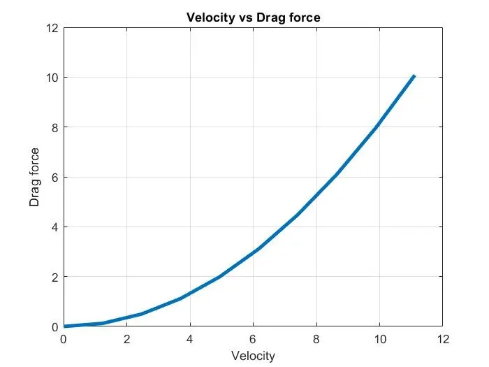
figure(1)
plot(V,Fd,'linewidth',3)
xlabel('Velocity')
ylabel('Drag force')
title('Velocity vs Drag force')
grid on

% program for drag coefficient and drag force

% Inputs
V   = 11.11;  
Cd  = linspace(.2486,0.3092,10);
Fd  = 0.5*rho*A*((V.^2)*Cd);
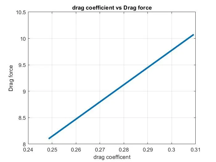
figure(2)
plot(Cd,Fd,'linewidth',3)
xlabel('drag coefficent')
ylabel('Drag force')
title('drag coefficient vs Drag force')
grid on 

code explanation

• First, the program is given a comment- then the basic commands like clear all, close all, and clc are used
• The required data for calculation of the code is added, like values of V, A, etc.
• The formulas used to calculate the drag force Fd are also typed in.
• the velocity (V) is assumed to be 40kmph which when converted is about 11.11m/s.
• to plot the graph between velocity and drag force 10 values are taken from 0 to 11.11 using the linspace command.
• these values are sued to calculate the drag force for the various velocities, and the acquired values are plotted using the plot command. The X and Y axis are labeled accordingly and a title is given to the plot.
• The value for Cd- drag coefficient is taken between 0.2486 and 0.3092 based on a study paper on the internet.
• The plot for drag coefficient and the drag force is calculated next (figure 2) and the drag coefficient is varied from 0.2486 to 0.3092 for 10 values using the linspace command.
• the results are plotted using a plot command and the X and Y axis labeled accordingly. The plot is given a title using the title command.

results and graphs