Code for solving an Air standard Cycle and calculating the thermal Efficiency using MATLAB
Objective
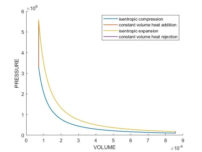
To write a code to solve an otto cycle and make plots for it and to calculate the thermal efficiency
Solution
- An otto cycle is used in a petrol internal combustion engine to produce work.
- it has mainly 4 processes or cycles
- Adiabatic compression(1-2)- Air and fuel mixture are compressed isentropically inside the cylinder.
- Constant volume heat addition (2-3)- Combustion takes place inside the cylinder due to the addition of an external source of heat/ignition
- Adiabatic expansion(3-4)- high pressure and high-temperature gasses expand inside the cylinder
- Constant volume heat rejection(4-1)- exhaust gasses are pushed out from the cylinder and the process is completed and the cycle is repeated.
Required inputs have to be provided using basic thermodynamic formulas in the code and save the required output, and make an adiabatic curve by using the calling function.
Function code is as follows:
% engine Kinematics function code

function [V]= engine_kinematics1(bore,stroke,con_rod,cr,start_crank,end_crank)

a =stroke/2;
R = con_rod/a;

%swept and clearance volume calculations

v_s= (pi/4)*bore^2*stroke;
v_c=v_s/(cr-1);

theta= linspace(start_crank,end_crank,100);

%combustion volume calculations in parts

term1= 0.5*(cr-1);
term2= R+1 - cosd(theta);
term3= (R^2-sind(theta).^2).^0.5;

V=(1+ term1*(term2-term3)).*v_c;

end
Code explanation
- The function is established and the values are defined for the various components like stroke, con rod length, etc.
- an array is created for theta using the linspace command.
- the various formulas are defined in 3 terms and in the end, all of them are combined together to make the function(V) work.
Code for PV diagram and Thermal Efficiency
clear all
close all
clc

%inputs
gamma=1.4;
t3=2300;

%state variables
p1=101325
t1=500

%engine parameters

bore=0.1;
stroke=0.1;
con_rod=0.15;
cr=12;

% calculating swept and clearance volumes
v_swept=(pi/4)*bore^2*stroke
v_clearance= v_swept/(cr-1);

v1=v_swept+v_clearance;
v2= v_clearance

%state variables at state2
%p2*v2^gamma=p1v1^gamma
%p2= p1*(v1/v2)^gamma
p2= p1*cr^gamma;


%p1v1/t1=p2v2/t2 | t2=(p2*v2*t1)/(p1*v1);
 t2=(p2*v2*t1)/(p1*v1);

constant_c=p1*v1^gamma;
 V_compression= engine_kinematics1(bore,stroke,con_rod,cr,180,0);
P_compression=constant_c./V_compression.^gamma;

 %state at point 3
 v3=v2;
 %(p3v3)/t3==(p2v2)/t2 |p3==p2*(t3/t2);
 p3=p2*(t3/t2);


constant_c=p3*v3^gamma;
 V_expansion= engine_kinematics1(bore,stroke,con_rod,cr,0,180);
P_expansion=constant_c./V_expansion.^gamma;

 %variable at point 4
 v4=v1;

 %p3v3^gamma==p4v4^gamma
 p4 = p3*(v3/v4)^gamma;

 %thermal efficiancy
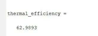
 thermal_efficiency=(1-(1/cr^(gamma-1)))*100

 figure(1)
 hold on

plot(V_compression,P_compression,'linewidth',1.25)
plot([v2,v3],[p2,p3],'linewidth',1.25)
plot(V_expansion,P_expansion,'linewidth',1.25)
plot([v4,v1],[p4,p1],'LineWidth',1.25)

xlabel('VOLUME')
ylabel('PRESSURE')
legend('isentropic compression','constant volume heat addition','isentropic expansion','constant volume heat rejection')
Code explanation
- The code is started using the basic commands like close all, clear all, and clc
- the input variables are added i.e. gamma.
- the state variables and the engine parameters are entered which include the stroke, bore, etc.
- The swept and clearance volumes are calculated.
- pressure and volume are calculated at point 2.
- calculating the V_compression by calling up the function and also P_compression.
- calculating the pressure and volume at points 3. and 4.
- then calculating the thermal efficiency using the formula (1-(1/cr^(gamma-1)))*100
- Then using the plot command to plot the PV diagram
- using the label command to label the x and y axis accordingly
- A legend command was also used to explain the different processes going on in the plot
Errors faced while programming
Basic typo errors were solved by checking and observing the code.
RESULTS:
Outputs
Thermal efficiency
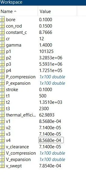
Workspace
PV diagram