Week 5 - Genetic Algorithm
1.AIM:
Optimize salagamite function by using genetic algorithm for the global maxima of the function.
2.THEORY:
Optimization:
- Optimization is the process of selection from the set of values for the imposed targets and the constraints.
- process handling mayny parameters ,where its integrated with each other and afffects one another in all aspects.
- It is been very dificult to manage and select the appropriate range of values for the defined targets and constraints.
- To make this process ease,optimization technique helps us to find a way to get the best out of it.
Stalagmite function:
- A stalagmite is an upward-growing mound of mineral deposits that have precipitated from water dripping onto the floor of a cave. Most stalagmites have rounded or flattened tips.
- A stalagmite function generally refers to the function with which we are generating values over a stalagmite kind of surface for finding out the local and global maxima and minima of that particular given function.
Population algorithms:
- An algorithm that maintains an entire set of candidate solutions,and each solution corresponds to a unique point in the search space of the problem known as population base algorithm.
Applications of optimization:
- Mechanics
- Economis and finance
- Machine learning
- Artificial intelligence
- Controls Engineering
Genetic algorithm:
- Provides effecient ,effective technique for optimization and machine learning applications.
- widely used today in business ,scientific and engineering circles.
Process Flow of genetic algorithm:
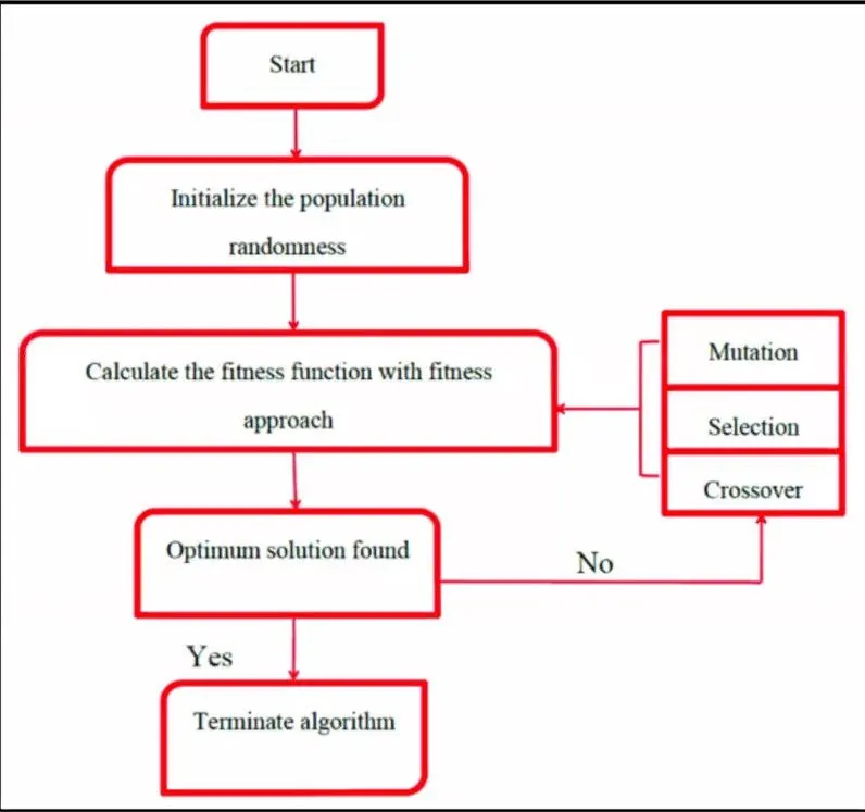
- The flowchart explains the working of genetic algorithm.
- The three main processes going behind the GA solvers such as:
1.Selection
2.Crossover
3.Mutation
Outline of the Algorithm:
- Creating a random initial population .
- Creates a sequence of new populations .
- Scores each member of the current population by computing its fitness value.
- Select members,called parents,based on their fitness value.
- At each step ,the genetic algorithm uses the current population to create the children that make up the next generation.
- The algorithm selects a group of individuals in the current population ,called parents.
- The algorithm usually selects individuals that have better fitness values as parents.
Creating next generation:
- Selection:It defined the selection of parents for the next generation using selection function/fitness function which will be based on the fitness value.
- Cross over:Crossover enables the algorithm to extract the best characters from different individuals and recombine them into potentially superior children.
- Mutation:Mutation adds to the diversity of a population and thereby increases the likelihood that the algoritm will generate individuals with better fitness values.
- Types of children produced for next generation from the current population parents as follows:
1.Elite child:Individuals having best fitness values.
2.Crossover child:Created by combining the parents.
3.Mutation child:Created by doing random changes to the single parent.
GA Syntax:
x=ga(fun,nvars,A,b,Aeq,beq,lb,ub,nonlcon,options)
Where fun= objective function.
nvar= number of variables.(specified as positive integers)
A,b=linear inequality constraints (A=Real matrix ,b=real vector)
Aeq,beq= Linear equality constraints (A=Real matrix ,b=real vector)
Lb,ub= Lower bounds and upper bounds
nonlcon= Nonlinear constraints
options= Optimization options
3.PROGRAM DESCRIPTION:
1.In this program we will first give x an y array by using linspace command here it is like x=linspace(0,0.6,150);
Matlab Main Code:
clear all
close all
clc

x=linspace(0,0.6,150);
y=linspace(0,0.6,150);
% creating a two dimensional mesh
[xx yy]=meshgrid(x,y);
%evaluating the stalagmite function
for i=1:length(xx)
    for j=1:length(yy)
        input_vector(1)=xx(i,j);
        input_vector(2)=yy(i,j);
        f(i,j)=stalagmite(input_vector);
    end
end

num_cases=50 % GA runs for 50 iterations
tic          % Study Time count start
% Study-1 statistical behaviour
for i=1:num_cases
    [inputs,fopt(i)]=ga(@stalagmite,2); % GA function is used to run the stalagmite data and give the optimal solutions.
    xopt(i)=inputs(1);
    yopt(i)=inputs(2);
    optf(i)=-fopt(i)     %Ga gives us Minima value.Inverse f_opt is taken for Maxima value
end
study1_time = toc     % Study Time count end


figure(1)
subplot(2,1,1)
hold on
surfc(xx,yy,-f) %Generation of stalagmite function.
shading interp   % To bring visually smooth curve surface without mesh lines
plot3(xopt,yopt,optf,'marker','o','MarkerSize',5,'MarkerFaceColor','r')  %plotting the optimum values with a red dot marker along the stalagmite 3D curves
title('unbounded inputs')
subplot(2,1,2)
plot(optf)              %plot of opt_f for every iterations
xlabel('iterations')
ylabel('function maximum')

    tic    % Study Time count start
    % Study 2-statistical behaviour with upper and lower bounds
    for i=1:num_cases
        [inputs,fopt(i)]=ga(@stalagmite,2,[],[],[],[],[0;0],[1,1]);  % GA function is used to run the stalagmite data and give the optimal solutions.
        xopt(i)=inputs(1);
        yopt(i)=inputs(2);
        optf(i)=-fopt(i)        %Ga gives us Minima value.Inverse f_opt is taken for Maxima value
    end
    study2_time=toc           % Study Time count end
    figure(2)
    subplot(2,1,1)
    hold on
    surfc(xx,yy,-f)        %Generation of stalagmite function.
    shading interp         % To bring visually smooth curve surface without mesh lines
    plot3(xopt,yopt,optf,'marker','o','MarkerSize',5,'MarkerFaceColor','r')
    title('bounded inputs')
    subplot(2,1,2)
    plot(optf)             %plot of opt_f for every iterations
    xlabel('iterations')
    ylabel('function maximum')

    tic        % Study Time count start

% Study-3 increasing GA iterations
options=optimoptions('ga');   % optimoptions is used to increase population size
options=optimoptions(options,'populationsize',  170);

 tic

    for i=1:num_cases
        [inputs,fopt(i)]=ga(@stalagmite,2,[],[],[],[],[0;0],[1,1],[],[],options);  % GA function is used to run the stalagmite data and give the optimal solutions.
        xopt(i)=inputs(1);
        yopt(i)=inputs(2);
        optf(i)=-fopt(i)      %Ga gives us Minima value.Inverse f_opt is taken for Maxima value
    end
    study3_time=toc           % Study Time count end
    figure(3)
    subplot(2,1,1)
    hold on
    surfc(xx,yy,-f)         %Generation of stalagmite function.
    shading interp          % To bring visually smooth curve surface without mesh lines
    plot3(xopt,yopt,optf,'marker','o','MarkerSize',5,'MarkerFaceColor','r')
    title('bounded inputs with increased population size')
    subplot(2,1,2)
    plot(optf)            %plot of opt_f for every iterations
    xlabel('iterations')
    ylabel('function maximum')
Matlab Function Code:
function [f]=stalagmite(input_vector)
x=input_vector(1);
y=input_vector(2);
f1x=(sin((5.1*pi*x)+0.5))^6;
f1y=(sin((5.1*pi*y)+0.5))^6;
f2x=exp(-4*log(2)*(((x-0.0667)^2)/0.64));
f2y=exp(-4*log(2)*(((y-0.0667)^2)/0.64));
f=-(f1x*f1y*f2x*f2y);
end
Error Rectification:
- While execution of code error occured because meshgrid not created while coding i.e.

- While plotting the surface negative sign of function is not used due to which there is a mismatch between points and surface. corrected by changing f to -f in surf command .
Output:
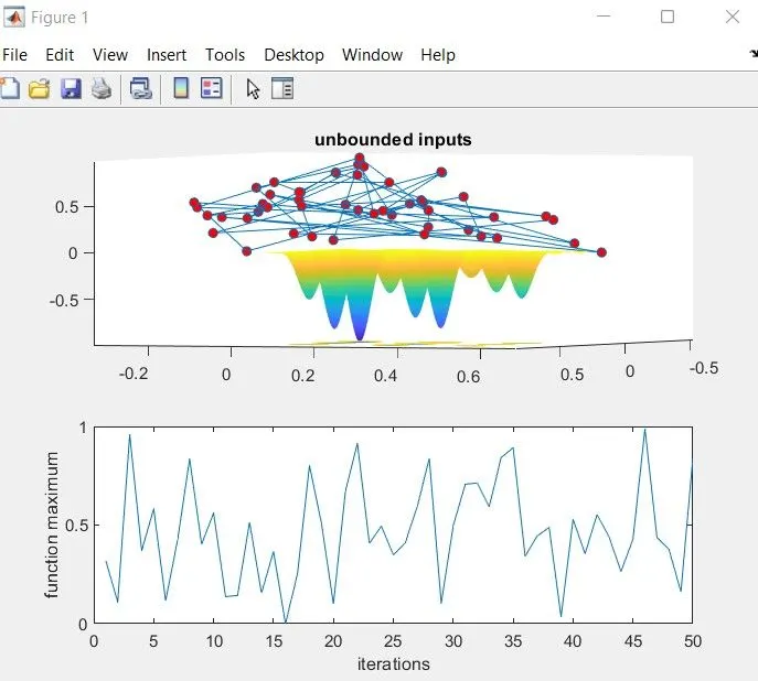
STATISTICAL STUDY WITHOUT BOUNDATION:
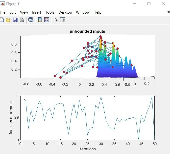
In this case as we can clearly see the optimized results are not accurate and there are so many data points on the graph.
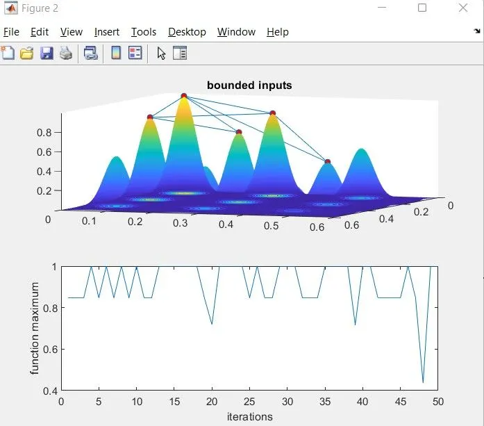
STATISTICAL STUDY WITH BOUNDATION:
- By providing the upper and the lower limit in the ga the search space is reduced with the upper and lower boundary.
- After providing boundary limits the optimum value variation is reduced to the previous case.
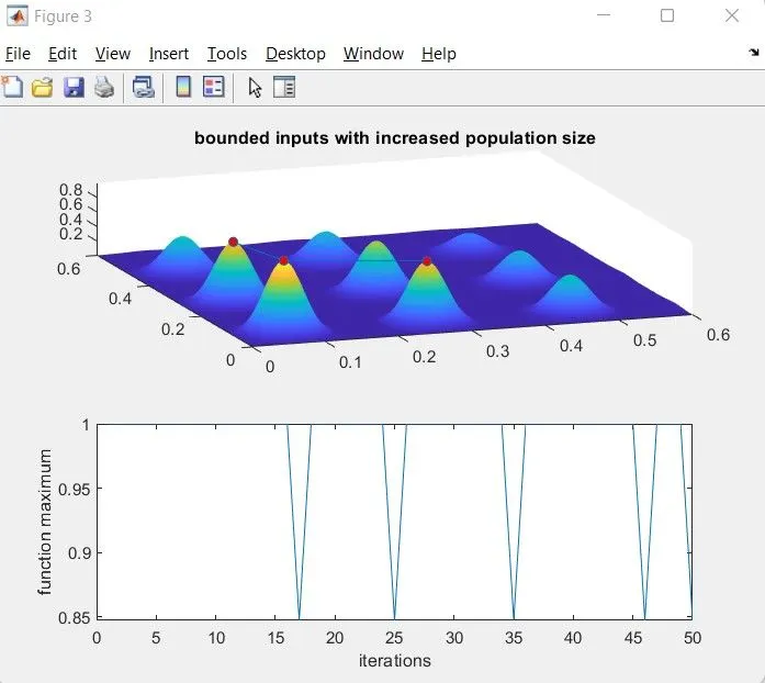
STATISTICAL STUDY WITH INCREASE IN SIZE OF POPULATION:
- Here as we have increased the size of the population ,so that the large numbers will provide better solutions.
- It is observed that the optimum points are rduced and we will be having better solutions compared to previous cases.
4.CONCLUSION:
- We can find out the optimum complex solution by using matlab by giving input data in x and y formats.
- With providing boundary counditions to the function ,it has improved drastically and we were closer to the solution.
- By increasing the iterations we can find out the optimum value of any function .This method can be used to find optimum solution.
5.REFERENCES: