Plotting of Otto cycle using MATLAB

1.AIM:Plot a PV diagram for otto cycle and calculate the thermal efficiency of Otto cycle using MATLB.

2.THEORY:This cycle is so named as it was conceive by ‘Otto’.On this cycle ,petrol ,gas and many types of oil engines work.It is the standard of comparison for internal combustion engines.

Fig(a) and fig(b) shows the theoretical P-v and T-s diagram of this cycle respectively.

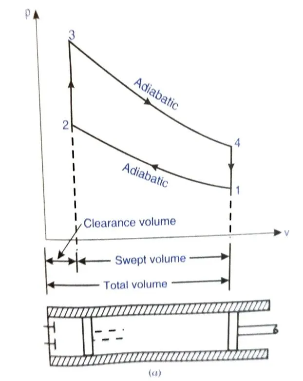
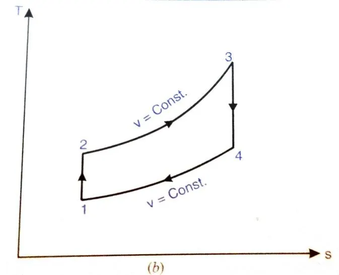
• Process(1-2):It represents adiabatic compression process.
• Process(2-3):It represents constant volume heat addition.
• Process(3-4):It represents adiabatic expansion process.
• Process(4-1):It represents constant volume heat rejection process.

  Governing Equations:

• Process (1-2) and Process(3-4): Both these processes are adiabatic and on P-v diagram are represented by equation

Where P is the pressure of the working fluid,V is the volume and `γ` is the specific heat ratio respectively.

• P-V-T Relations: we can find the p,v,t relations by using ideal gas equation

PV=nRT ,where P is pressure , V is volume ,R is gas constant , T is temperature , n is number of moles of gas .

• For calculating swept volumeand clearance volume:
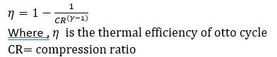
• Thermal efficiency: For otto cycle thermal efficiency is given by

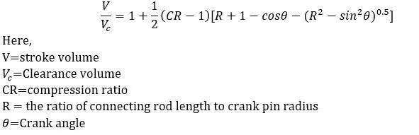
• Piston Kinematics analysis: The piston kinematics tells us the how piston moves from TDC to BDC , also describes how the chamber volume changes with function of time .Piston kinematics equation is given as

3.PROGRAM DESCRIPTION:

• In this program first we will give some input values like `γ`,temperature at state 3, pressure at state 1 and temperature of state1 .These values are given for the calculation of the other state points of different states by using the above equations of constant volume and adiabatic processes.
• Initially we will also give input of some engine parameters like bore of cylinder,stroke ,connecting rod length and compression ratio .These values are given for the calculation of swept volume ,clearance volume etc.
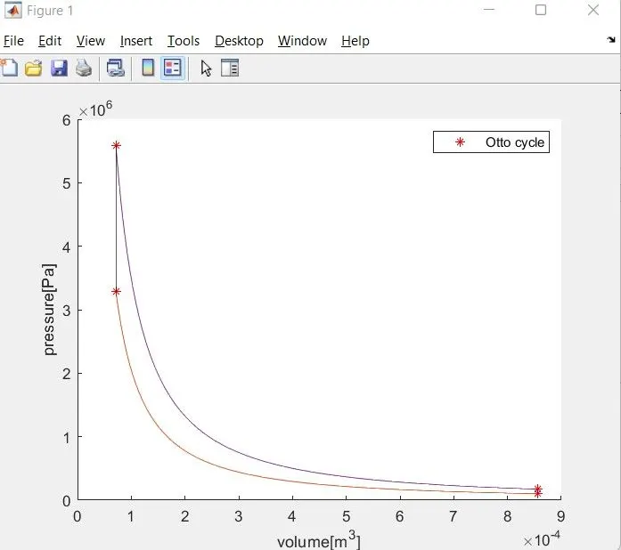
• By using the properties at 4 states like , pressure , volume and temperature we can plot the four states on the P-V diagram .
• To get the variation of volume with the various values of crank angle now we will write a function code named as (engine_kinematics) and we will use this code for the two adiabatic processes to trace the variation of Volume (V) with crank angle (`θ`).
• Now we will calculate the thermal efficiency of the otto cycle by using themal efficiency equation .(mentioned above).
• At the end we will plot all the points and variation on the P-V diagram to get a plot.

Matlab Main Code:
clear all
close all
clc
%input  
gamma=1.4
t3=2300
%state variables
p1=101325
t1=500
%engine geometric parameters
bore=0.1;
stroke=0.1;
con_rod=0.15;
cr=12;
%calculating the swept volume and the clearance volume
v_swept=(pi/4)*bore^2*stroke;
v_clearance=v_swept/(cr-1);

v1=v_swept+v_clearance
v2=v_clearance

%state variables at state point 2
%p2v2^gamma=p1v1^gamma
%p2=p1*(v1/v2)^gamma=p1*cr^gamma
p2=p1*cr^gamma;

%p1v1/t1=p2v2/t2|t2=p2*v2*t1/(p1*v1)
t2=p2*v2*t1/(p1*v1)
constant_c=p1*v1^gamma
v_compression=engine_kinematics(bore,stroke,con_rod,cr,180,0);
p_compression=constant_c./(v_compression.^gamma)
%state variables at state point 3
v3=v2
%p3v3/t3=p2v2/t2|p3=p2*t3/t2
p3=p2*t3/t2


constant_c=p3*v3^gamma
v_expansion=engine_kinematics(bore,stroke,con_rod,cr,0,180);
p_expansion=constant_c./(v_expansion.^gamma)

%state variables at state4
v4=v1
%p3v3^gamma=p4v4^gamma| p4=p3(v3/v4)^gamma
p4=p3*(v3/v4)^gamma

%calculation of thermal efficiency
thermal_efficiency=1-1/(cr^(gamma-1))

figure(1)
hold on
plot(v1,p1,'*','color','r')
plot(v_compression,p_compression)
plot(v2,p2,'*','color','r')
plot(v_expansion,p_expansion)
plot(v3,p3,'*','color','r')
plot(v4,p4,'*','color','r')
plot([v2 v3],[p2 p3],'color','k')
plot([v4 v1],[p4 p1],'color','b')
xlabel('volume[m^3]')
ylabel('pressure[Pa]')
legend('Otto cycle')

Matlab Function Code:
function [v]=engine_kinematics(bore,stroke,con_rod,cr,start_crank,end_crank)
a=stroke/2
R=con_rod/a
v_s=pi/4*bore^2*stroke;
v_c=v_s/(cr-1);
theta=linspace(start_crank,end_crank,100);
term1=0.5*(cr-1);
term2=R+1-cosd(theta);
term3=(R^2-sind(theta).^2).^0.5;
v=(1+term1*(term2-term3)).*v_c;
end

Error Rectification:

• This error occurred because of typing error while defining the value for variable con_rod , we have written con_ro .spelling corrected code rectified.

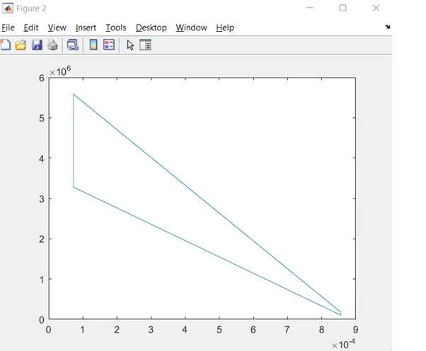
• Initially when the variation of volume is not considered with the variation in crank angle ,so we got plot like that mentioned below .Then the variation is taken into consideration and graph corrected.

Output:

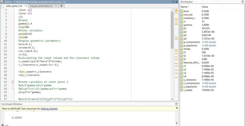
• When the code get executed all the properties of different state point ,thermal efficiency and the P-V diagram will be displayed.

• We will also get a P-V diagram showing all the four states of the otto cycle and the variation in different properties with crank angle.

4.CONCLUSION:

• We observed that by varying the input parameters and crank angle we observed the variation in the different state points of the otto cycle.
• We can calculate thermal efficiency of the otto cycle by using this Matlab program.
• We can also find the net work from the area under P-V diagram.