Week 4.1 - Solving second order ODEs
SIMPLE PENDULUM:
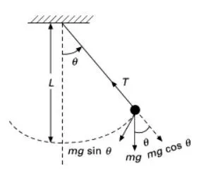
The simple pendulum is another mechanical system that moves in an oscillatory motion. It consists of a point mass ‘m’ suspended by means of light inextensible string of length L from a fixed support as shown in Fig.The motion occurs in a vertical plane and is driven by a gravitational forces.
1.AIM:
- To write a program that solves the ODE ,representing the equation of motion of a simple pendulum with damping.
- To create a plot between angular velocity,angular displacement w.r.t. time.
- To make an animation video(simulation) of the motion of the pendulum.
2.THEORY:
A pendulum is a weight suspended from a pivot so that it can swing freely. When a pendulum is displaced sideways from its resting, equilibrium position, it is subject to a restoring force due to gravity that will accelerate it back toward the equilibrium position. When released, the restoring force acting on the pendulum's mass causes it to oscillate about the equilibrium position, swinging back and forth. The time for one complete cycle, a left swing and a right swing, is called the period. The period depends on the length of the pendulum and also to a slight degree on the amplitude, the width of the pendulum's swing.
The way the pendulum moves depends on the Newtons second law. When this law is written down, we get a second order Ordinary Differential Equation that describes the position of the "ball" w.r.t time.
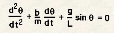
This ODE represents the equation of motion of a simple pendulum with damping:
where
g = gravity in m/s2,
L = length of the pendulum in m,
m = mass of the ball in kg,
b=damping coefficient.
Governing Equations:
This equation is a second order differential equation and we have to convert it into first order.
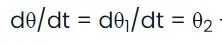
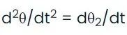
To conert we will assume ,let us consider:
 ........(1)
 ..........(2)
 ......................(3)
By using these assumptions we can reduce the above second order equation as folllows:
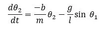
so we have broken second order ODE equation to two first order ODE.
and then we will form a matrix like this:
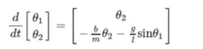
ODE45-Syntax:
[t,y] = ode45(odefun,tspan,y0)tspan = [t0 tf], integrates the system of differential equations y′=f(t,y) from t0 to tf with initial conditions y0. Each row in the solution array y corresponds to a value returned in column vector t.here odefun is the derivative function.
3.PROGRAM DESCRIPTION:
- In this program first we will give some input values like damping coeeficient ,acceleration due to gravity,length of pendulum , mass of bob ,initial velocity in rad/sec,initial dispacement .
- we will make a function program and create an ode function which will be called while using it in the main program.
- The inputs are for the simple pendulum are specified and the b = damping coefficient = 0.05 (n-m/s), g = acceleration due to gravity = 9.81 (m/s^2), l = length of the string = 1(m), m = mass of the bob = 1 (kg).
- t_span is used here which specifies the time span of the iterations that are going to solve the ordinary differential equation.
- ode45 is a function in MATLAB that solves ordinary or partial differential equations using a numerical method. In this problem the highest order is 2. So, we have to take two constant values so that the equation is changed to simple differential equation.
- Syntax of ODE45 is :
[t,results]=ode45(@(t,theta) ode_func(t,theta,b,g,l,m),t_span,theta_0)
- Figure 1 is showing how the damping is taking place for the pendulum. The angular velocity and displacement will come to rest at end of the function.
- Plot command is used to plot the time and angular velocity/angular dispalacement.
- The label command is used to label the X & Y axis.
- Legend command is used to label the angular velocity and the displacement.
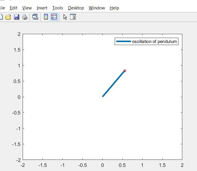
- For loop is used to trace the motion of pendulum at different points and the plot is created in figure 2, which is a simulation .
- Initial point of pendulum is taken x0,y0 and the changing position is x1,y1.
- To make the movie we have used certain commands as follows:M(ct)=getframe(gcf)
getframe:it captures the figure as frame.
gcf:it refers to the current figure handle in matlab.
counter variable:it helps in indexing of frames sequence.
Movie(M):plays the movie frames in array 'M' once.
videowriter:this creates a video file of specified name and format.
open:opens the specified file(video file)
writevideo:writes the created video file with the frames captured in the 'M' array.
close:closes the specified file.
and then the video file will be saved in the program path.
Matlab Main code:
clear all
close all
clc

% b=damping coefficient
b=0.05;
% g=acc due to gravity in m/s^2
g=9.81;
% l=length of pendulum in m
l=1;
% m=mass of bob in kg
m=1;
% initial condition of pendulum
% initial velocity v=3 rad/s ,initial displacement =0
theta_0=[0;3];
%time values
t_span=linspace(0,20,500);
%solve ODE
[t,results]=ode45(@(t,theta) ode_func(t,theta,b,g,l,m),t_span,theta_0);
figure(1)
plot(t,results(:,1))
hold on
plot(t,results(:,2))
title('motion of pendulum')
ylabel('Angulat velocity(rad/s)/Displacement(rad)')
xlabel('time(sec)')
legend('displacement','angular velocity')

angle=results(:,1)

ct = 1
for i=1:length(angle)
    ANGLE=angle(i);
    x0=0;
    y0=0;
    x1=l*sin(ANGLE);
    y1=-l*cos(ANGLE);
     %plotting
     figure(2)

       plot([x0 x1],[y0 y1],'LineWidth',3)
        hold on
       plot(x1,y1,'*','color','r')
       axis([-2 2 -2 2])
       legend('oscillation of pendulum')
        pause(0.03)
        M(ct)=getframe(gcf);
        ct=ct+1;
        hold off

end
movie(M)
videofile=VideoWriter('oscillation of pendulum.avi','Uncompressed AVI');
open(videofile)
writeVideo(videofile,M)
close(videofile)
Matlab Function code:
function [dtheta_dt]=ode_func(t,theta,b,g,l,m)
theta1=theta(1)
theta2=theta(2)
dtheta1_dt=theta2;
dtheta2_dt=(-b/m)*theta2-(g/l)*sin(theta1);
dtheta_dt=[dtheta1_dt;dtheta2_dt];
end
Error Rectification:
- This error occurred because of typing error while defining the value for variable dtheta_dt, we have written dtheta-dt .spelling corrected code rectified.

- We have taken the value of y1=l*cos(ANGLE); due to which pendulum motion was not adequate.Then it was corrected as y1=-l*cos(ANGLE).
Output:
- A plot is created between the angular acceleration and displacement of the motion of simple pendulum along with time ,here as to the time passes the anngular velocity and angular displacement goes on decreasing and it becomes equivalent to zero at the end.
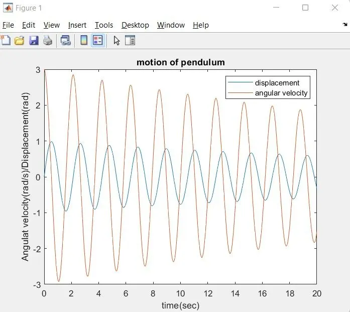
- Here blue line represents the displacement and red line represents the angular velocity.
4.CONCLUSION:
- We observed that ODE45 solver can be used to solve one degree diferential equation having one of its variable varying with time.
- We observed the variation in the output of the angular velocity and displacement w.r.t time how it goes on decreasing because of damping and by changing the input parameters the graph changes significantly.
- Simulation of pendulum is made to observe the motion and how it get damped with time.
Youtube link of animation: