Week 5 - Genetic Algorithm

OBJECTIVE:

• Write a code in MATLAB to optimise the stalagmite function and find the global maxima of the function.
• Clearly explain the concept of genetic algorithm in your own words and explain the syntax for ga in MATLAB in your report.
• Make sure that your code gives the same output, even if it is made to run several times.
• Plot graphs for all three studies and for F maximum vs no. of iterations. Title and axes labels are necessary; legends could be shown if necessary.

THEORY:

GENETIC ALGORITHM(GA):

The genetic algorithm, based on natural selection, the mechanism that propels biological evolution, is a technique for resolving both limited and unconstrained optimization issues. The genetic algorithm repeatedly modifies a population of unique solutions. The genetic algorithm chooses members of the present population to serve as parents at each stage and employs them to produce the offspring that will make up the following generation. The population "evolves" through generations towards an optimal solution.

Flow Chart:

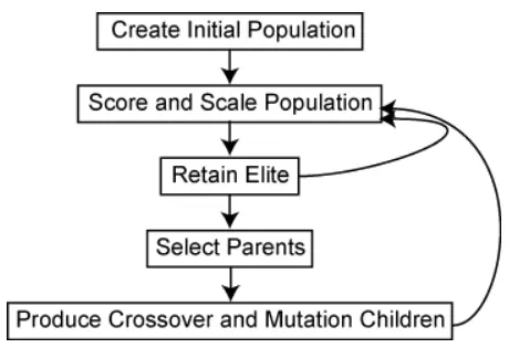
Source: MATLAB Documentation

Steps:

The following phases are considered in a genetic algorithm:

1. Initialization: The process begins with a set of individuals called a Population. Each individual is a solution to the problem.
2. Fitness Function: based on an individual's ability to compete with others, a raw fitness score is given to each member of the population.
3. Selection: Two sets of people (parents) are chosen based on their fitness ratings. High-fitness people are more likely to be chosen for reproduction.
4. Crossover: The process of recombining the genetic components of the chosen individuals to create new children.
5. Mutation: is the process of introducing random variations into the progeny in order to increase population diversity.
6. Termination: If the population does not produce children considerably different from the previous generation, the algorithm terminates.

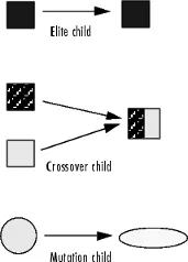
Source: MATLAB Documentation

Syntax:

This is the general syntax in MATLAB for GA:

[x,fval,exitflag,output,population,scores] = ga(fun,nvars,A,b,Aeq,beq,lb,ub,nonlcon,intcon,options)

where,

fun = objective function
nvars = number of variables
A, b = Linear Inequality Constraints such that, A*x <= b
Aeq, beq = Linear Equality Constraints such that, Aeq*x = beq
lb = lower bounds
ub = Upper bounds
nonlcon = Non-Linear constraints
options = Optimisation option to change limits, tolerances, population size etc.
intcon = integer variables
x = solution vector
fval = optimised value of the function returned by ga
exitflag = returns the reason for GA termination
output = shows information about the optimisation process
population = final population matrix
scores = column vector of final scores

STALAGMITE FUNCTION:

We define a stalagmite function as:

This will act as our fitness function; our goal is to optimise the function and calculate the global maxima. To compute the function, we will create a stalagmite.m function, which we will use in our main code:

function result = stalagmite(input)

x = input(1); 
y = input(2);

f_1x = (sin(5.1*pi*x + 0.5))^6;
f_1y = (sin(5.1*pi*y + 0.5))^6;
f_2x = exp(-4*log(2)*((x-0.0667)^2/0.64));
f_2y = exp(-4*log(2)*((y-0.0667)^2/0.64));

result = -(f_1x*f_2x*f_1y*f_2y); # -ve to calculate maxima
end

Note that Genetic Algorithm minimises a given function. Therefore, to calculate the maxima, we will multiply the resulting function with the '-' sign. This will result in the maxima value being the minimum value, and we can use GA as it is.

CODE:

We will conduct three studies - Unconstrained, Constrained and with a Larger Population Size.

FITNESS FUNCTION:

First, we write the code to create our fitness function and plot the stalagmite function:

% Optimisation using Genetic Algorithm

close all    % Close all plots
clear        % clear workspace
clc          % clear commands

% Creating sample space:
x = linspace(0,0.6,150);
y = linspace(0,0.6,150);

[xx,yy] = meshgrid(x,y); % Grid Space

% Evaluate local maxima and minima using stalagmite function
for i = 1:length(x)
    for j = 1:length(y)
        input_vector(1) = xx(i,j);
        input_vector(2) = yy(i,j);
        f(i,j) = stalagmite(input_vector);
    end
end

% Plot local Maxima and Minima
surf(x,y,-f) 
shading interp  % Hide Gridlines

Output:

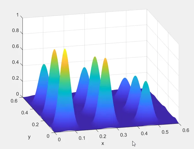
Note that we are plotting '-f' to show the actual plot since we have multiplied the function with '-'.

STUDY 1: UNCONSTRAINED OPTIMISATION:

In unconstrained optimisation, we let the GA do all the guessing. It automatically generates random inputs to provide based on the fitness function and works its way towards optimisation:

%% Study 1 - Unconstrained Optimisation:     
        
tic;             % Start time
iteration = 50;  % Number of Iterations for GA
rng default;     % for reproduciblity

% Calculating Optimised Value using GA:
for i=1:iteration
    
    [inputs,fopt(i)]=ga(@stalagmite,2);    
    xopt(i)=inputs(1);                      
    yopt(i)=inputs(2);
    
end
study1_time=toc; % End Time
    
% Plotting:
figure(2)

subplot(2,1,1)
surfc(xx,yy,-f);      
hold on
shading interp

plot3(xopt,yopt,-fopt,'marker','o','markersize',5,'markerfacecolor','r');
xlabel('x');
ylabel('y');
grid on

subplot(2,1,2)
plot(-fopt);
xlabel('iterations')
ylabel('function max value')

Output:

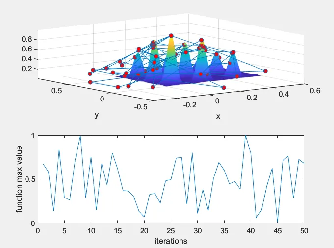
We can infer from these outputs that the results are incoherent and completely random, and some values lie beyond our area of interest (Sample Space). This is because the GA assumes all random values and works on that basis. To help it, we will constrain the region between the maximum and minimum values of the domains.

STUDY 2: CONSTRAINED OPTIMISATION:

In constrained optimisation, We set the constraints bwtween which GA is allowed to guess for valid inputs. This greatly improves the accuracy. To set the constraints, we will use the lb and ub parameters of GA and set the lowest limit as 0 and upper limits as 0.6 according to our sample space. We will leave the other parameters blank since we don't need them:

%% Study 2 - Constrained Optimisation:


tic;  % Start time

% Calculating Optimised Value using GA:
for i=1:iteration
    
    [inputs,fopt(i)]=ga(@stalagmite,2,[],[],[],[],[0;0],[0.6;0.6]);   
    xopt(i)=inputs(1);                                           
    yopt(i)=inputs(2);
    
 end
study2_time=toc;  % End Time
    
% Plotting:
figure(3)

subplot(2,1,1)
hold on
surfc(xx,yy,-f)
shading interp

plot3(xopt,yopt,-fopt,'marker','o','markersize',5,'markerfacecolor','r');
xlabel('x');
ylabel('y');
grid on

subplot(2,1,2)
plot(-fopt);
xlabel('iterations')
ylabel('function max value')

Output:

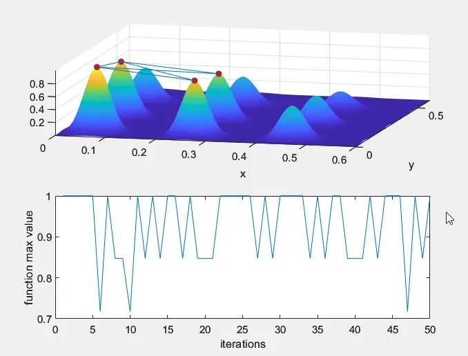
As we can see from these outputs, the result is much more accurate, and the algorithm determines the maximum between these four peaks. The frequency of deviating from the actual maxima has also reduced.

STUDY 3: INCREASING POPULATION SIZE:

To further improve the results, we increase the initial population size, which improves the resolution of the solution and thus increases accuracy. We will use a population size of 400 and use the options parameter to define it:

%% Study 3 - Increasing the Population Size

tic;  % Start Time
options=optimoptions('ga','populationsize',400); % Specifying Population Size         

% Calculating Optimised Value using GA:
for i=1:iteration
    
    [inputs,fopt(i)]=ga(@stalagmite,2,[],[],[],[],[0;0],[0.6;0.6],[],[],options);
    xopt(i)=inputs(1);
    yopt(i)=inputs(2);         
     
end
study3_time=toc;
    
% Plotting:
figure(4)

subplot(2,1,1)
hold on
surfc(xx,yy,-f)
shading interp

plot3(xopt,yopt,-fopt,'marker','o','markersize',5,'markerfacecolor','r');
xlabel('x');
ylabel('y');
grid on

subplot(2,1,2)
plot(-fopt);
xlabel('iterations')
ylabel('function max value')

Output:

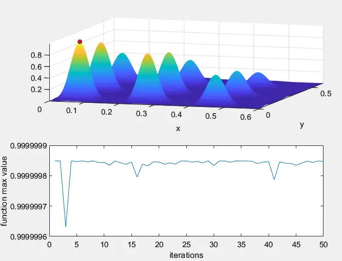
From these results, it's clear that the algorithm is much more accurate now. It points to the peak; on the other hand, the value is also accurate up to the 6th decimal, which is very precise and accurate.

MAXIMA VS NUMBER OF ITERATIONS:

Now we will increase the number of iterations and see its effect on the third study:

Iteration = 75:

Iteration = 100:

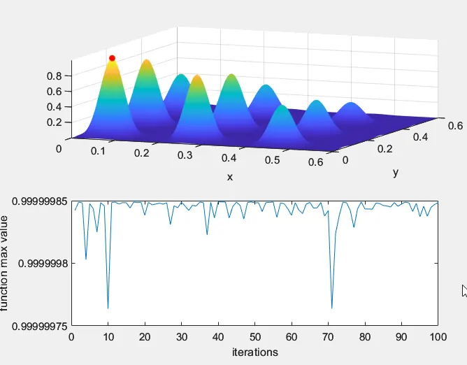
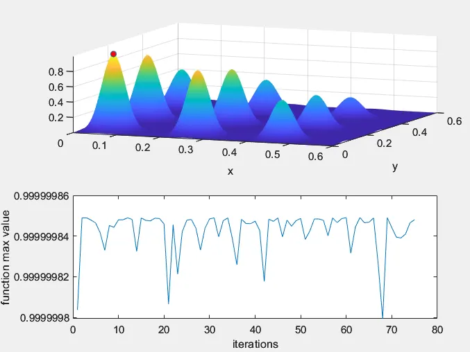
As we increase the number of iterations, the precision increases considerably, and the fluctuation magnitude is reduced. However, it comes at a temporal cost, as doubling the number of iterations doubles the run time.

CONCLUSION:

• GA by itself will not produce accurate results. Some inputs are necessary to make the problem more specific to arrive at an accurate solution.
• Increasing the population size considerably increases the run time. A similar effect is observed by increasing the number of iterations.
• An optimum solution can be developed by varying the number of iterations and the population size to arrive at an accurate solution in minimal time.

REFERENCES:

1. MATLAB DOCUMENTATION. <What is Genetic Algorithm?>
2. MEDIUM: Towards Data Science. <Introduction to Genetic Algorithms — Including Example Code>
3. MATLAB DOCUMENTATION. <GA help>