Week 5 - Curve fitting

Title:

Thermodynamic Curve Fitting Analysis: A Python-Based Approach.

Aim:

The aim of this study is to analyze thermodynamic data and model the relationship between temperature (T) and specific heat capacity (Cp) using curve fitting techniques implemented in Python.

Objectives:

• To fit mathematical models to experimental data for characterizing the T-Cp relationship.
• To evaluate the fitness characteristics of the fitted curves.
• To analyze the implications of the curve fitting analysis on understanding thermodynamic behavior.

Solution:

We propose a Python-based solution utilizing curve fitting techniques to model the T-Cp relationship. The solution involves the following steps:

• Data acquisition: Obtain experimental data on temperature and specific heat capacity.
• Curve fitting: Fit mathematical models, such as linear and cubic functions, to the experimental data using the curve_fit function from the SciPy library.
• Evaluation: Assess the fitness characteristics of the fitted curves, including SSE, SSR, SST, R^2, and RMSE.
• Analysis: Analyze the implications of the curve fitting analysis on understanding thermodynamic behavior.

Procedure:

• Import the necessary libraries: NumPy, Matplotlib, and SciPy.
• Define the curve fitting functions for linear and cubic models.
• Read thermodynamic data from a file.
• Fit curves to the data using curve-fitting functions.
• Evaluate fitness characteristics: SSE, SSR, SST, R^2, and RMSE.
• Plot the experimental data and fitted curves.
• Analyze the results and discuss the implications.

Results & Discussion:

1. What do popt and pcov mean?

Popt and Pcov:

• Popt is a numpy array containing the optimized parameters (coefficients) of the curve fit. These parameters are estimated by the curve fitting algorithm to minimize the difference between the fitted curve and the actual data.

• Pcov is the estimated covariance of popt. It represents the uncertainty or error associated with each parameter estimate. The diagonal elements of pcov provide the variances of the parameter estimates.

2. What does np.array (temperature) do?

np.array(temperature):

• It converts the list or array temperature into a numpy array. This conversion is often done to utilize the capabilities and functions provided by Numpy, which are optimized for array operations and mathematical computations.

3. What does the * in *popt mean?

The * in popt:

• The * in *popt is the unpacking operator in Python. It is used to unpack the elements of the popt array (or tuple) and pass them as individual arguments to a function. In the context of curve fitting, *popt passes the optimized parameters as separate arguments to the curve fitting function.

4. Write code to fit a linear and cubic polynomial for the Cp data. Explain if your results are good or bad.

# -*- coding: utf-8 -*-
"""
Created on Mon Apr  8 12:34:46 2024

@author: zeusm
"""

import numpy as np
import matplotlib.pyplot as plt
from scipy.optimize import curve_fit

# Define curve fit functions

def linear_function(t, a, b):
    return a * t + b

def cubic_function(t, a, b, c, d):
    return a * t**3 + b * t**2 + c * t + d

# Read thermodynamic data from file

def read_data(filename):
    temperature, cp = [], []
    with open(filename, 'r') as file:
        for line in file:
            t, data = map(float, line.split(','))
            temperature.append(t)
            cp.append(data)
    return np.array(temperature), np.array(cp)

# Fit curve and plot data

def plot_data_fit(temperature, cp, fit_func, fit_label):
    popt, pcov = curve_fit(fit_func, temperature, cp)
    fit_cp = fit_func(temperature, *popt)
    plt.plot(temperature, cp, 'k--', label='Actual data')
    plt.plot(temperature, fit_cp, color='red', linewidth=1, label=fit_label)
    plt.xlabel('Temperature (K)')
    plt.ylabel('Cp')
    plt.legend()
    plt.show()
    return fit_cp

# Measure fitness characteristics

def measure_fitness(cp, fit_cp):
    mean_cp = np.mean(cp)
    sse = np.sum((cp - fit_cp) ** 2)
    ssr = np.sum((fit_cp - mean_cp) ** 2)
    sst = sse + ssr
    r_squared = ssr / sst
    rmse = np.sqrt(sse / len(cp))
    return sse, ssr, sst, r_squared, rmse

# Main program

def main():
    temperature, cp = read_data('data')
    
    # Linear curve fitting
    fit_cp_linear = plot_data_fit(temperature, cp, linear_function, 'Linear curve fit')
    linear_sse, linear_ssr, linear_sst, linear_r_squared, linear_rmse = measure_fitness(cp, fit_cp_linear)
    print("Linear curve fit:")
    print(f"SSE: {linear_sse}")
    print(f"SSR: {linear_ssr}")
    print(f"SST: {linear_sst}")
    print(f"R^2: {linear_r_squared}")
    print(f"RMSE: {linear_rmse}\n")

    # Cubic curve fitting
    fit_cp_cubic = plot_data_fit(temperature, cp, cubic_function, 'Cubic curve fit')
    cubic_sse, cubic_ssr, cubic_sst, cubic_r_squared, cubic_rmse = measure_fitness(cp, fit_cp_cubic)
    print("Cubic curve fit:")
    print(f"SSE: {cubic_sse}")
    print(f"SSR: {cubic_ssr}")
    print(f"SST: {cubic_sst}")
    print(f"R^2: {cubic_r_squared}")
    print(f"RMSE: {cubic_rmse}")

if __name__ == "__main__":
    main()

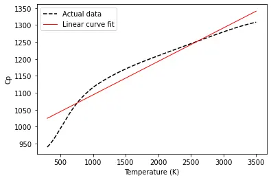
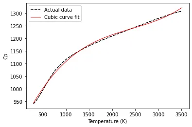
• When the actual relationship between the variables is non-linear, such as in the case where the data follows a cubic form, attempting to fit a linear model may not capture the underlying pattern adequately.
• In contrast, using a higher-degree polynomial model, such as a cubic polynomial, allows for a more flexible curve fit that can better capture the non-linear relationship between the variables.

5. What needs to be done in order to make the curve fit perfectly?

To achieve a perfect curve fit, several factors need to be considered and potentially addressed:

• Model Selection: Choose the most appropriate mathematical model that accurately represents the underlying relationship between the variables. This may involve exploring various model forms (linear, polynomial, exponential, etc.) and selecting the one that best fits the data.
• Data Quality: Ensure high-quality and precise experimental data. Minimize measurement errors, outliers, and missing values in the dataset.
• Initial Guesses: Provide reasonable initial guesses for the parameters of the curve fitting model. These initial guesses can significantly impact the convergence and accuracy of the optimization algorithm.
• Optimization Algorithm: Select an appropriate optimization algorithm for curve fitting. Different algorithms may converge to different solutions, and some may be more suitable for specific types of models or datasets.
• Parameter Constraints: Apply constraints on the parameters of the model if necessary, to ensure that they remain within physically meaningful ranges.
• Regularization: Apply regularization techniques to prevent overfitting and improve the generalization ability of the model.
• Evaluation and Validation: Evaluate the goodness of fit using appropriate metrics (e.g., R^2, RMSE) and validate the model against independent datasets or reference values.

6. Show empirically how well your curve has been fit.

Metrics	Linear Curve Fit	Cubic Curve Fit
Sum of Squared Errors (SSE)	2163049.089	94272.021
Sum of Squared Residuals (SSR)	26630624.160	28699401.236
Sum of Squared Total (SST)	28793673.250	28793673.256
Coefficient of Determination (R^2)	0.925	0.997
Root Mean Square Error (RMSE)	25.999	5.428

Physical Significance:

• SSE (Sum of Squared Errors): Measures the overall discrepancy between the fitted curve and the actual data points. Lower values indicate a better fit.
• SSR (Sum of Squared Residuals): Quantifies the variance explained by the model. Higher values suggest that the model captures more variability in the data.
• SST (Sum of Squared Total): Represents the total variability in the observed data. It is the sum of the variance explained by the model and the unexplained variance.
• Coefficient of Determination (R^2): Indicates the proportion of variability in the dependent variable explained by the independent variable through the fitted model. Higher values denote a better fit.
• RMSE (Root Mean Square Error): Measures the average magnitude of errors between the fitted curve and the actual data points. Lower values indicate a better fit, as the model's predictions are closer to the observed values on average.

Conclusion:

• In summary, these metrics provide a comprehensive assessment of the curve-fitting models' performance, including their ability to capture the data's variability and predictability.