Week 5 - Curve fitting
1)
popt means parameters optimised, arbitary constants of functions are optimised using curve fitting. For example:
import numpy as np
from scipy.optimize import curve_fit
import matplotlib.pyplot as plt
# Example data
x_data = np.array([1, 2, 3, 4, 5])
y_data = np.array([2.1, 4.1, 6.2, 8.2, 10.1])
def fit_curve(x,a,b,c):
return a*pow(x,2)+b*x+c
# Perform curve fitting
popt, pcov = curve_fit(fit_curve, x_data, y_data)
print(popt)
output:
[-0.02142857 2.13857143 -0.04 ]
pcov means parameter covarience, covarience describes about the change of one parameter with respect to another. Smaller the covarience, better the fitting.
import numpy as np
from scipy.optimize import curve_fit
import matplotlib.pyplot as plt
# Example data
x_data = np.array([1, 2, 3, 4, 5])
y_data = np.array([2.1, 4.1, 6.2, 8.2, 10.1])
def fit_curve(x,a,b,c):
return a*pow(x,2)+b*x+c
# Perform curve fitting
popt, pcov = curve_fit(fit_curve, x_data, y_data)
print(pcov)
output:
[[ 0.00016327 -0.00097959 0.00114286]
[-0.00097959 0.00610612 -0.00754285]
[ 0.00114286 -0.00754285 0.01051427]]
2)np.array(temperature):
np refers to numpy library which is used for numerical computing
np.array(temperature) refers to creating an array for temperature attributes.
3)*popt:
This command is used call the optimised parameters into the function, calculated using cure_fit.
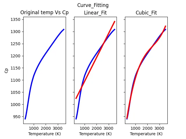
Write code to fit a linear and cubic polynomial for the Cp data. Explain if your results are good or bad.
What needs to be done in order to make the curve fit perfect?
Show empirically as to how well your curve has been fit.
import matplotlib.pyplot as plt
import numpy as np
from scipy.optimize import curve_fit
def func_1(t,a,b):
return a*t+b
def func_2(t,a,b,c):
return a*pow(t,2)+b*t+c
def func_3(t,a,b,c,d):
return a*pow(t,3)+b*pow(t,2)+c*t+d
def func_4(t,a,b,c,d,e):
return a*pow(t,4)+b*pow(t,3)+c*pow(t,2)+d*t+e
def read_file():
temperature = []
cp = []
for line in open('data','r'):
values = line.split(',')
temperature.append(float(values[0]))
cp.append(float(values[1]))
return[temperature,cp]
temperature,cp = read_file()
def CF(func,temp,cp):
popt,pcov = curve_fit(func,temperature,cp)
fit_cp = func(np.array(temperature),*popt)
return fit_cp,popt,pcov
def GoF(t,cp,func,popt):
print("Mean Squared Error:",np.mean((cp-func(np.array(temperature),*popt)**2)))
ss_res = np.dot((cp-func(np.array(t),*popt)),(cp-func(np.array(t),*popt)))
y_mean = np.mean(cp)
ss_total = np.dot((cp-y_mean),(cp-y_mean))
print('R-square value:',1-(ss_res/ss_total))
fit_cp_linear,popt,pcov = CF(func_1,temperature,cp)
print('Goodness of fit for linear polynomial:')
GoF(temperature,cp,func_1,popt)
print()
fit_cp_cubic,popt,pcov = CF(func_3,temperature,cp)
print('Goodness of fit for cubic polynomial:')
GoF(temperature,cp,func_3,popt)
print()
fig, ax = plt.subplots(1,3,sharex=True,sharey=True)
fig.suptitle('Curve_Fitting')
ax[0].plot(temperature,cp,color='blue',linewidth=3)
ax[0].set_title('Original temp Vs Cp')
ax[1].plot(temperature,cp,color='blue',linewidth=3)
ax[1].plot(temperature,fit_cp_linear,color='red',linewidth=3)
ax[1].set_title('Linear_Fit')
ax[2].plot(temperature,cp,color='blue',linewidth=3)
ax[2].plot(temperature,fit_cp_cubic,color='red',linewidth=3)
ax[2].set_title('Cubic_Fit')
for A in ax.flat:
A.set(xlabel='Temperature (K)',ylabel='Cp')
for A in ax.flat:
A.label_outer()
plt.show()
output:
Goodness of fit for linear polynomial:
Mean Squared Error: -1406121.2622456765
R-square value: 0.9248776260551824
Goodness of fit for cubic polynomial:
Mean Squared Error: -1406767.7550853402
R-square value: 0.9967259467140538
R-Square value is about 0.997. The high R-Square value indicates that the cubic fit explains approximately 99.7% of the data's variability