Week 5 - Curve fitting

01. popt refers to optimizing parameters defined in an equations and these variables will be obtained using curve_fit function

pcov refers to co-variance matrix for the above popt values

02. np.array(temperature) will pass the complete array of temperature values into the functions and it makes sure that values for every temperature output is generated.

03. * in *popt refers to assigning the unknown constants in an equation generated from curve_fit function.

04.

Objective:

To Write a Python code for plotting a linear and cubic equation to fit a Cp tempearture data. Also to calculate the the errors using appropriate methods and evaluate best fit.

Solution Procedure:

What is Curve Fitting ?

Curve fitting is the process of constructing a curve, or mathematical functions, which possess the closest proximity to the real series of data. By curve fitting, we can mathematically construct the functional relationship between the observed dataset and parameter values, etc. It is highly effective in the mathematical modeling of some natural processes.

Assume data points (x1,y1) , (x2,y2) , (x3,y3) , ... (xn,yn) and assume the best fit for these set of points will be y = f(x), the criterion under which the equation of the curve will be the best fit possible is as follows,

Suppose each of these n points has an individual error (difference in y co-ordinate values)

The error for a general "i" point can be given by the function,

Error=|y(i)−value of f(x) at x(i)|=|y(i)−f(x(i))|Error=|y(i)-value of f(x) at x(i)|=|y(i)-f(x(i))|

To remove the modulus sign, it is effective if we square the error term, when we square the error terms and add the errors for all the 'n' points we get,

SSE(sum of squared errors)=n∑i=1Error(i)2SSE(sum of squared errors)=∑i=1nError(i)2

assume the proposed equation is a nth degree polynomial of the form,

f(x)=A1+A2⋅x+A3⋅x2+...+An⋅xn−1f(x)=A1+A2⋅x+A3⋅x2+...+An⋅xn-1

How to choose the best fit?

Upon finding a curve which satisfies the data points there are 4 quantities which help us measure the goodness of fit criteria or how well the equation is a representing the datapoints. There are,

• The sum of squares due to error (SSE)
• R-square
• Adjusted R-square
• Root mean squared error (RMSE)

The first quantity SSE was already measured in the previous section of this article,

• R-square

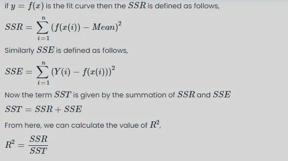
This quantity that measures how successful the fit is in explaining the variation of the data. Put another way, R-square is the square of the correlation between the response values and the predicted response values. It is also called the square of the multiple correlation coefficient and the coefficient of multiple determination.

What that means in layman's terms is that the higher the value of R-square the better the fit, the lower it is the lousier the fit, R-square ranges from a value of 0 to 1

• 0 for the worst possible fit for the data set
• 1 for the best possible fit for the data set

The value of R-square can be calculated using the following formula,

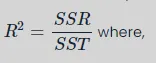
SSR = sum of squares of the regression, which is basically the square of the difference between the value of the fitting function at a given point and the arithmetic mean of the data set.

• Adjusted R-square

Adjusted R-square is a normalizing variation of R-square which neglects the variation of R-square due to insignificant independent variables.

for, y=f(x1,x2,x3,...,xn)y=f(x1,x2,x3,...,xn), here, x1,x2,...,xnx1,x2,...,xn are the independent variables and yy is the dependent variable.

• If value of x(i)x(i) contributes to the output yy, then x(i)x(i) is a significant dependent variable
• If value of x(i)x(i) does not contribute to the output yy, then x(i)x(i) is an insignificant dependent variable

What that essentially explains is demonstrated below with an example,

Assume a linear fit with the data as given below,

Now, let us assume we add another variable to this same case,

Since we transpose a 2d plot into 3d plot the discreet datapoints will become a line function showing no variation about the 3rd axis(Weight of Chef).

The 2d regression function will become a plane with no variation about the 3rd axis(Weight of Chef).

From here and logically, it is intuitive that the new variable "Weight of Chef" will have little to no effect on the Cost of the pizza. But still, it is observed that the R-square new increases.

So, in conclusion, as long as you keep adding new variables into any system, even if they may seem completely unrelated, they will still be related to the system in an infinitesimally small manner.

This is the reason the adjusted R-square is required.

Adjusted R-square disregards these infinitesimally small increments to R-square, and only considers the variables which actually contribute to the output of the system in a drastic way.

R-square is formulated as shown below,

where,

n - the number of datapoints

k - the number of independent variables

• RMSE (Root Mean Squared Error)

This statistic is also known as the fit standard error and the standard error of the regression. It is an estimate of the standard deviation of the random component in the data, and is defined as,

where,

n is the total number of datapoints available.

Using these four quantities Matlab effectively deduces the goodness of fit, typically is R-square is greater than 0.95 the fit is assumed to be good.

Python Code:

# Writing a program to fit a curve for an linear equation and cubic equation for temp vs cp
# To find out the best fit for the ideal curve
# Project By: Shivakumar G R

# Defining the libraries

import math
import matplotlib.pyplot as plt
import numpy as np
from scipy.optimize import curve_fit

# Defining a linear curve fit function
def linear_func(t,a,b):
	return a*t+b

# Defining a cubic equation for curve fit
def cubic_func(t,a,b,c,d):
	return a*pow(t,3)+b*pow(t,2)+c*t+d


# Function to read data from file
def read_file():
	t=[]
	cp=[]
	for line in open ('data','r'):
		value=line.split(',')
		t.append(float(value[0]))
		cp.append(float(value[1]))
	return[t,cp]


# Function to calulate the fit errors

def error_func(temp,cp,fcp):
	sse=0
	ssr=0
	m=np.mean(cp)
	for i in range(len(cp)):
		sse+=pow((cp[i]-fcp[i]),2)
		ssr+=pow((cp[i]-m),2)
	sst=sse+ssr
	r_square=(ssr/sst)
	rmse=pow((sse/len(cp)),0.5)
	return(sse,r_square,rmse)

temp,cp=read_file()

# In order to get better curve fit we will split the values of cp into multiple set of numbers

cp1=cp[0:800]
cp2=cp[800:1600]
cp3=cp[1600:2400]
cp4=cp[2400:3200]

temp1=temp[0:800]
temp2=temp[800:1600]
temp3=temp[1600:2400]
temp4=temp[2400:3200]


# Calling a linear function

popt_l,pcov_l=curve_fit(linear_func,temp,cp)
fit_curve_lin=linear_func(np.array(temp),*popt_l)

popt_l1,pcov_l1=curve_fit(linear_func,temp1,cp1)
fit_curve_lin1=linear_func(np.array(temp1),*popt_l1)

popt_l2,pcov_l2=curve_fit(linear_func,temp2,cp2)
fit_curve_lin2=linear_func(np.array(temp2),*popt_l2)

popt_l3,pcov_l3=curve_fit(linear_func,temp3,cp3)
fit_curve_lin3=linear_func(np.array(temp3),*popt_l3)

popt_l4,pcov_l4=curve_fit(linear_func,temp4,cp4)
fit_curve_lin4=linear_func(np.array(temp4),*popt_l4)

#Finding out the accuracy of fit using error calculations

sse_l,r_square_l,rmse_l=error_func(temp,cp,fit_curve_lin)

print('sum of square of error for a linear curve is:',sse_l)
print('R Square value for linear equation:',r_square_l)
print('Root Mean Squared Error for linear equation:',rmse_l)

if (r_square_l<0.95):
	print('The linear equation is not a perfect fit for the curve')
else:
	print('The linear equation is a perfect fit for the curve')

#Calling a cubic function 

popt_c,pcov_c=curve_fit(cubic_func,temp,cp)
fit_curve_cub=cubic_func(np.array(temp),*popt_c)

popt_c1,pcov_c1=curve_fit(cubic_func,temp1,cp1)
fit_curve_cub1=cubic_func(np.array(temp1),*popt_c1)

popt_c2,pcov_c2=curve_fit(cubic_func,temp2,cp2)
fit_curve_cub2=cubic_func(np.array(temp2),*popt_c2)

popt_c3,pcov_c3=curve_fit(cubic_func,temp3,cp3)
fit_curve_cub3=cubic_func(np.array(temp3),*popt_c3)

popt_c4,pcov_c4=curve_fit(cubic_func,temp4,cp4)
fit_curve_cub4=cubic_func(np.array(temp4),*popt_c4)

#Finding out the accuracy of fit using error calculations

sse_c,r_square_c,rmse_c=error_func(temp,cp,fit_curve_cub)

print('sum of square of error for a cubic curve is:',sse_c)
print('R Square value for cubic equation:',r_square_c)
print('Root Mean Squared Error for cubic equation:',rmse_c)

if (r_square_c<0.95):
	print('The cubic equation is not a perfect fit for the curve')
else:
	print('The cubic equation is a perfect fit for the curve')


# Plotting all the data obtained by above calculations

plt.plot(temp,cp,'r',label='Ideal Curve',linewidth=3)
plt.plot(temp1,fit_curve_lin1,'g',label='Linear equation fit curve',linewidth=2)
plt.plot(temp2,fit_curve_lin2,'g',linewidth=2)
plt.plot(temp3,fit_curve_lin3,'g',linewidth=2)
plt.plot(temp4,fit_curve_lin4,'g',linewidth=2)
plt.plot(temp1,fit_curve_cub1,'b--',label='Cubic polynomial equation fit curve')
plt.plot(temp2,fit_curve_cub2,'b--')
plt.plot(temp3,fit_curve_cub3,'b--')
plt.plot(temp4,fit_curve_cub4,'b--')
plt.xlabel('Temperature  --->',c='b')
plt.ylabel('Cp --->',c='b')
plt.legend(loc='lower right')
plt.savefig('Curvefitting.png')
plt.show()

05. In order to have better curve fit we can split the array of elements into multiple arrays so that we can evaluate a bettr curve fit. so in order to achieve this in our coding we have split the array into four arrays and evaluate the data.

06. In order to show that our curve fit is be good or bad we have calculated the R_square Values to show our curve is good or bad and same we have evaluated through coding.

We havce claculated the R square values to show how good is our fit.

Results and conclusion:

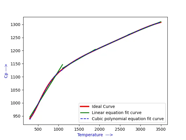
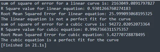
After running the code and plotting the data we could able conclude that a cubic polynomial function is best fit where as linear function is not.

the R Square value for linear function found to be 0.93 which is less than 0.95 that the ideal value to identify best fit.

where as with cubic polynomial equation we got R square value 0.99 which can be concluded as good fit

Hence Cubic polynomial function is a best fit for cp vs temeprature curve fit.