Week 2 Air standard Cycle

Objective:

1. write and execute a python code that calculates and plot a P-V diagram for otto cycle.

2. Calculating thermal efficiency of otto cycle in the end using calculated temperature parameters and print the output.

Problem Statement:

We have a otto cycle with following geometric dimensions and inputs.

Inputs
p1=101325 Pa
t1=500 K
t3=2300 K
c_r=12
gamma=1.4

Engine geometry parameters
bore=0.2
stroke=0.2
con_rod=0.3

Using the above parameters we need to plot a otto cycle diagram in P-V plot. and thermal efficiency to be calculated.

Brief Introduction:

An Otto cycle is a idealized thermodynamic cycle that describes the functioning of a typical spark ignition piston engine. It is the thermodynamic cycle most commonly found in automobile engines.

The Otto cycle is a description of what happens to a gas as it is subjected to changes of pressure, temperature, volume, addition of heat, and removal of heat. The gas that is subjected to those changes is called the system. The system, in this case, is defined to be the fluid (gas) within the cylinder. By describing the changes that take place within the system, it will also describe in inverse, the system's effect on the environment. In the case of the Otto cycle, the effect will be to produce enough net work from the system so as to propel an automobile and its occupants in the environment.

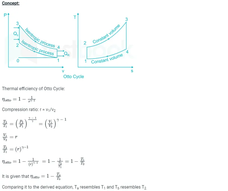
The processes are described by:

• Process 0–1 a mass of air is drawn into piston/cylinder arrangement at constant pressure.
• Process 1–2 is an adiabatic (isentropic) compression of the charge as the piston moves from bottom dead center (BDC) to top dead center (TDC).
• Process 2–3 is a constant-volume heat transfer to the working gas from an external source while the piston is at top dead center. This process is intended to represent the ignition of the fuel-air mixture and the subsequent rapid burning.
• Process 3–4 is an adiabatic (isentropic) expansion (power stroke).
• Process 4–1 completes the cycle by a constant-volume process in which heat is rejected from the air while the piston is at bottom dead center.
• Process 1–0 the mass of air is released to the atmosphere in a constant pressure process.

Solution Procedure:

Now we are intersested in plotting a pv diagram so we need to calculate pressure, volume and temperature at the end of each process in order to develop a cycle.

• Calculating p1,v1 and p2,v2 for isentropic compression

As we already have p1 as our atmospheric pressure and we can compute v1

v1=v_s+V_c

Where v_s is a swept volume which can be calculated using engine geometry as (pi/4)*bore^2*stroke

Clearance volume can be calculated using compression ratio as V_s/(c_r-1)

now to calculate p2 and v2

we know that at the end of compression volume will be equal to clearance volume. so,

v2=V_c

pressure is calculated using

p2=p1*v1^gamma/v2^gamma

• Calculating p3,v3 using ideal gas equation

Since it is a isochoric process volume remains constant. Hence,

v2=v3

and p3 can be calculated using ideal gas equation

p3*v3/t3=p2*v2/t2

• Calculating p4,v4 for an isentropic expansion process

Here v4= v1

p4=p3*v3^gamma/v4^gamma

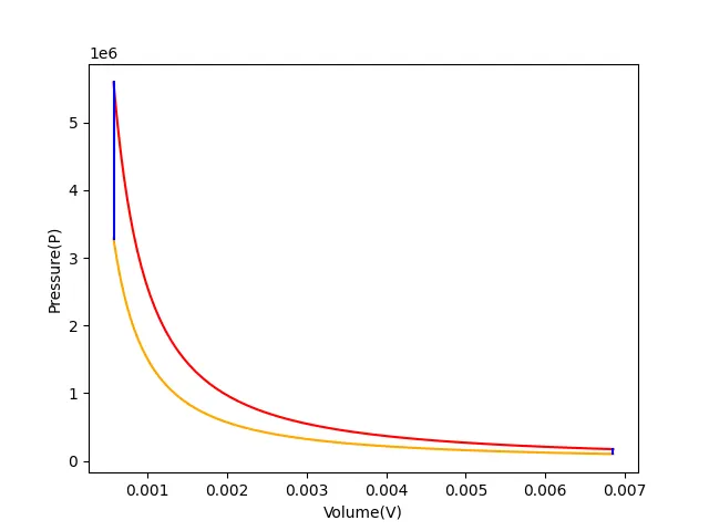
using all the above parametrs we can plot an otto cycle P-V Diagram using python

• Calculating Thermal Efficiency of otto cycle

We use following formala to calculate thermal efficency of an otto cycle.

Thermal efficiency=1-(t1/t2)

Python Code:

# Plotting a otto cycle curve using engine kinematics
#Project by: Shivakumar G R

# v/v_c=1+0.5*(c_r-1)[R+1-cos(theta)-(R^2-(sin(theta))^2)^0.5]

import math
import matplotlib.pyplot as plt
import numpy as np


#inputs
p1=101325
t1=500
t3=2300
c_r=12
gamma=1.4

#engine geometry parameters
bore=0.2
stroke=0.2
con_rod=0.3

#volume computation
v_s=math.pi*(1/4)*pow(bore,2)*stroke
v_c=v_s/(c_r-1)
v1=v_s+v_c

#Calculating R Value using formaulae | R=con_rod/a | where a=stroke/2
a=stroke/2
R=con_rod/a

# pressure array for storing compression and expansion values
p_comp=[]
p_exp=[]

def engine_kinematics(crank_start,crank_end):
	
	cs=math.radians(crank_start)
	ce=math.radians(crank_end)

	n=100

	crank_angle=np.linspace(cs,ce,n)
	V=[]
	for theta in crank_angle:
		
		term1=c_r-1
		term2=R+1-math.cos(theta)
		term3_1=(pow(R,2)-(pow(math.sin(theta),2)))
		term3=pow(term3_1,0.5)
		tmp_v=(1+0.5*term1*(term2-term3))*v_c
		V.append((1+0.5*term1*(term2-term3))*v_c)
		
	return(V)

v_comp=engine_kinematics(0,180)
for j in v_comp:
	rhs=p1*pow(v1,gamma)
	tmp_p=rhs/pow(j,gamma)
	p_comp.append(tmp_p)

#Calculating state points 2

v2=v_c

p2=p1*pow(v1,gamma)/pow(v2,gamma)

#Calculating state point 3
rhs=p1*v1/t1
t2=p2*v2/rhs
v3=v2
p3=rhs*t3/v3

#Calculating array of volume and pressure during isentropic expansion

v_exp=engine_kinematics(180,0)
for m in v_exp:
	rhs=p3*pow(v3,gamma)
	tmp_p=rhs/pow(m,gamma)
	p_exp.append(tmp_p)

# for calculating state points 4

v4=v1
p4=p3*pow(v3,gamma)/pow(v4,gamma)

# Calculating Thermal efficiency 

thermal_eff=1-(t1/t2)
print(thermal_eff)

plt.plot(v_comp,p_comp,"orange",label='Isentropic Compression')
plt.plot(v_exp,p_exp,"red",label='Isentropic Expansion')
plt.plot([v2,v3],[p2,p3],'blue',label='isochoric process')
plt.plot([v4,v1],[p4,p1],'blue')
plt.xlabel('Volume(V)')
plt.ylabel('Pressure(P)')
plt.savefig('engine_kinematics.png')
plt.legend()
plt.show()

Result:

The Calculated thermal efficiency for the engine is

0.6298928275128466

P-V Plot for otto cycle

Conclusion:

• Plotted P-V Diagram for an ooto cylcle.
• Calculated thermal efficiency for the cycle.