Week 3 - Solving second order ODEs

Objective:

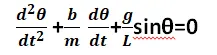
• Write a python program for solving second order ODE for a simple pendulum using

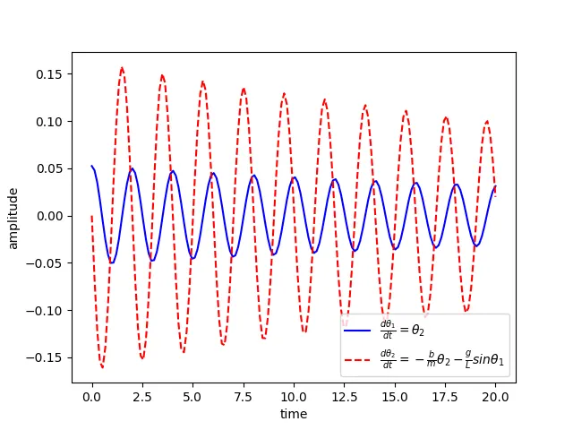
• After solving the second order ODE plot a graph for angular velocity and angular displacement against time varying from 0 to 20 seconds
• Also to simulate the simple pendulum oscillations using the above code.

Problem Statement:

A Second order Equation for harmonic motion of a simple pendulum has to be solved.

Using the above equation plots to be generated to simulate the simple pendulum motion.

Solution Procedure:

• For solving a second order ODE in python we need to break the equation into simple differential equation.

In order to achieve that we need to define the initial conditions i.e Initial angular displacement and initial velocity.

For current problem we assume that initial displacement is θ1

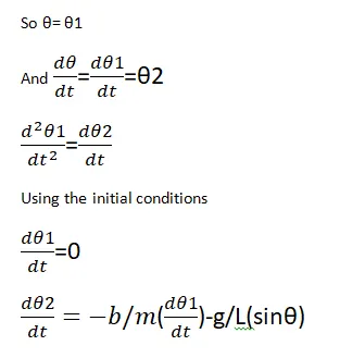
Using the above equations we will be solving the second order ODE in python using scipy library.

• For plotting the simple pendulum at various conditions to simulate the harmonic motion.

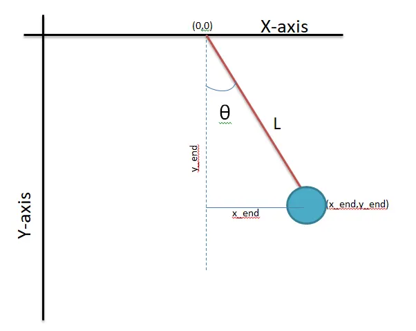
Calculation of x_end and y_end for respective θ value

x_end=L*sinθ

y_end=-L*cosθ

For each set of x_end ,y_end values we will be plotting the graph to make set of plots for the pendulum simulation.

Python Code:

# Solving second order ODE for simple pendulum
#Project By: Shivakumar G R

import math
import matplotlib.pyplot as plt
from scipy.integrate import odeint
import numpy as np

x_start=0
y_start=0
#inputs( damping co-efficient, gravity, lenght of pendulum, mass)
b=0.05
g=9.81
l=1
m=1
c_t=1



def dfdt(theta,t,b,g,l,m):
	theta_1=theta[0]
	theta_2=theta[1]
	

	dtheta1_dt=theta_2
	dtheta2_dt=((-b/m)*theta_2)-((g/l)*math.sin(theta_1))
	dtheta_dt=[dtheta1_dt, dtheta2_dt]

	return dtheta_dt


# initial conditions(velocity and displacement)
theta_disp=math.radians(3)
theta_0=[theta_disp,0]
# time points
t=np.linspace(0,20,150)

theta = odeint(dfdt,theta_0,t,args=(b,g,l,m))

#plotting the wave using integarted output

plt.plot(t,theta[:,0],'b-',label=r'$\frac{d\theta_1}{dt}=\theta_2$')
plt.plot(t,theta[:,1],'r--',label=r'$\frac{d\theta_2}{dt}=-\frac{b}{m}\theta_2-\frac{g}{L}sin\theta_1$')
plt.xlabel('time')
plt.ylabel('amplitude')
plt.legend(loc='best')
plt.savefig('Simple_pendulum.png')
plt.show()

# For creating plots fort simulation of pendulum
#Keeping one end stationery and other end points to be calculated
for i in theta[:,0]:

	x_end=l*np.sin(i)
	y_end=-l*np.cos(i)
	filename=str(c_t)+'.png'
	c_t = c_t+1

	plt.figure()
	plt.plot([-0.5,0.5],[0,0],'r',linewidth=3)
	plt.plot([0,0],[0,-1.5],'g--',linewidth=1)
	plt.plot([x_start,x_end],[y_start,y_end])
	plt.plot(x_end,y_end,'o',markersize=20)
	plt.xlim(-1.5,1.5)
	plt.ylim(-2,1)
	plt.savefig(filename)

Errors faced:

No such major errors were encountered while writing and executing a code.

Results and conclusions:

After writing and executing the code got a wave graph of angular displacement against time and it is observed that the amplitude the angular displacement gradually started decrease over the period of time.

and also after plotting angular velocity against time period same behaviour was observed.

After the plots are generated, all the plots were stitched to simulate the harmonic motion of a simple pendulum. Below is the link for the simulation video.

https://youtu.be/qn9wLz3Sy2k