Week 4.1 - Solving second order ODEs

Objective:

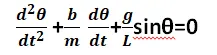
• Write a matlab program for solving second order ODE for a simple pendulum using

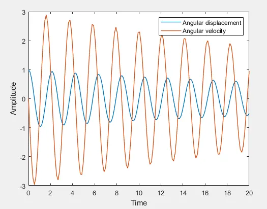
• After solving the second order ODE plot a graph for angular velocity and angular displacement against time varying from 0 to 20 seconds
• Also to simulate the simple pendulum oscillations using the above code.

Problem Statement:

A Second order Equation for harmonic motion of a simple pendulum has to be solved.

Using the above equation plots to be generated to simulate the simple pendulum motion.

Solution Procedure:

• For solving a second order ODE in Matlab we need to break the equation into simple differential equation.

In order to achieve that we need to define the initial conditions i.e Initial angular displacement and initial velocity.

For current problem we assume that initial displacement is θ1

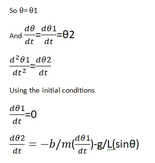
Using the above equations we will be solving the second order ODE in Matlab.

• For plotting the simple pendulum at various conditions to simulate the harmonic motion.

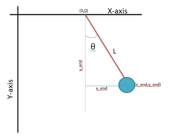
Calculation of x_end and y_end for respective θ value

x_end=L*sinθ

y_end=-L*cosθ

For each set of x_end ,y_end values we will be plotting the graph to make set of plots for the pendulum simulation.

Matlab Code:

% write a matlab code to plot harmonic motion of simple pendulum using ode
% integration

% Project By: Shivakumar G R

% Clearing the windows 
close all
clear all
clc

% Inputs for the program
b=0.05;
g=9.81;
l=1;
m=1;

% defining the initial conditions for the pendulum
theta_0=[1,0];
% Counter variable to store the frames for movie creation
ct=1;

% Starting our code by defining the time limit
t_span=linspace(0,20,150);

%Solving ODE function

[t,results]=ode45(@(t,theta) ode_func(t,theta,b,g,l,m),t_span,theta_0);


% Plotting the ode function with reference to time


figure(1)
plot(t,results(:,1),t,results(:,2),'linewidth',1)
xlabel('Time')
ylabel('Amplitude')
legend('Angular displacement','Angular velocity')

% defining the obtained data output for the animation
theta_1=results(:,l);
theta_2=results(:,2);

% demonstarting the animation of simple pendulum under above conditions.
figure(2)

% using for loop wel will calculate the position of pendulum at every point
% corresponding to its angular displacement
for i=1:length(theta_1)

   % Definign the fixed point for the pendulum string 
   x0=0;
   y0=0;

   % calculating the moving end of string for animation
   x_end=l*sin(theta_1(i));
   y_end=-l*cos(theta_1(i));
   
   % plotting the simple pendulum corresponding to its angular displacement
   plot([x0,x_end],[y0,y_end],[-0.7,0.7],[0,0],x_end,y_end,'-o','MarkerSize',25,'Markerfacecolor','m','markeredgecolor','m','linewidth',2)
   axis([-1.2,1.2,-1.5,1])
   pause(0.05)

   % storing the frames in a file M
   M(ct) = getframe(gcf);

   ct=ct+1;

end

%creating a movie file to write all frames and generate an animation

movie(M)
videofile=VideoWriter('simple_pendulum','uncompressed AVI');
open(videofile)
writeVideo(videofile,M)
close(videofile)

Matlab Function Code:

% Defining function to solve the second order ode for harmonic motion

function theta_s=ode_func(t,theta,b,g,l,m)
    % assignment of initial conditions
    theta_1=theta(1);
    theta_2=theta(2);

    % Calculating the results
    dtheta1=theta_2;
    dtheta2=-(b/m)*theta_2-(g/l)*sin(theta_1);
    % returning the values obtained to source file
    theta_s=[dtheta1;dtheta2];
end

Errors faced:

No such major errors were encountered while writing and executing a code.

Results and conclusions:

After writing and executing the code got a wave graph of angular displacement against time and it is observed that the amplitude the angular displacement gradually started decrease over the period of time.

and also after plotting angular velocity against time period same behaviour was observed.

Then program was executed to create a movie for animation of simple pendulum. Link for the AVI Video clip has been attached below.

https://youtu.be/1-eohBgc01E