Week 5 - Curve fitting
Curve fitting using python (linear and cubic curve fitting).
INTRODUCTION:-
Curve fit is a process of construction of curve , or mathematical function that
has a best fit to series of data points possibly subject to constraints. Curve
fitting can involve either interpolation whrere an exact fit to the data is required.
In this challege we will try to fit the linear and cubic polynomial to best fit the curve
obtained at the given data of temperature and specific heat at constant pressure(cp).
It is a statistical technique used to drive coefficient values for equations that express
the value for one (dependent) variable as a function of another(independent variable).
This is the engineering application in trend analysis, hypothesis testing, which is used
to compare existing mathematical model with measured data.
QUESTIONS:-
1) What does popt and pcov mean?
popt is an array with the optimal parameters obtained using a non linear least square-
fit.
pcov is a second array with the estimated covariance of the parameter in popt.
2) What does np.array(temperature) do?
A numpy array is a grid of values, all of the same type. Here it is being used to pass the
values of temperature to the function.
3) What does the * in *popt mean?
The star here means that is being referenced. Any and all change which could have occure
to popt while in a function would be reflected in the original popt.
5) What needs to be done in order to make the curve fit perfect?
A curve fit can almost never be perfect because experimental data will always vary from a
perfect equation. However the fit can be made as close as possible by trying different order
equations, extrapolation, dividing the data and curve fitting them seperately or on very rare
case finding an equation an equation which fits the data perfectly.
when we increased polynomial to get a perfect fit. But in this method we get a perfect curve
for a polynomial having very high order or split wise.
4) PROGRAM:-
import numpy as np
import matplotlib.pyplot as plt
from scipy.optmize import curve_fit
# curve fit function
def func( t, a, b ):
return a*t + b
# Reading thermodynamic data file
def read_file():
temperature = []
cp = []
for line in open( ' data(1)', 'r'):
values = line.split(',')
temperarure.append(float(values[0]))
cp.append(float(values[1]))
return [ temperature,cp]
# Main program
temperature, cp = read_file()
popt, pocv = curve_fit(func, temperature, cp)
fit_cp = func(np.array( temperature),*popt)
plt.figure(1)
plt.plot(temperature,cp, color = "blue", linewidth = 3)
plt.plot(temperature,fit_cp, color = "red", linewidth = 3)
plt.legend(['Actual data', 'curve'])
plt.xlabel('Temperature')
plt.ylabel('cp')
plt.show()
# Cubic curve fit function (cubic ploynomial)
def func( t, a, b, c ):
return a*pow(t,3) + b*pow(t,2) + c*t + d
# Reading thermodynamic data file
def read_file():
temperature = []
cp = []
for line in open( ' data(1)', 'r'):
values = line.split(',')
temperarure.append(float(values[0]))
cp.append(float(values[1]))
return [ temperature,cp]
# Main program
temperature, cp = read_file()
popt, pocv = curve_fit(func, temperature, cp)
fit_cp = func(np.array( temperature),*popt)
plt.figure(2)
plt.plot(temperature,cp, color = "blue", linewidth = 3)
plt.plot(temperature,fit_cp, color = "red", linewidth = 3)
plt.legend(['Actual data', 'cubic curve fit'])
plt.xlabel('Temperature [K]')
plt.ylabel('cp')
plt.show()
FOR PERFECT FIT PROGRAM:-
def func( t, a, b, c, d, e ):
return a*pow(t,4) + b*pow(t,3) + c*pow(t,2) + d*t + e
# Reading thermodynamic data file
def read_file():
temperature = []
cp = []
for line in open( ' data(1)', 'r'):
values = line.split(',')
temperarure.append(float(values[0]))
cp.append(float(values[1]))
return [ temperature,cp]
# Main program
temperature, cp = read_file()
popt, pocv = curve_fit(func, temperature, cp)
fit_cp = func(np.array( temperature),*popt)
plt.figure(2)
plt.plot(temperature,cp, color = "blue", linewidth = 3)
plt.plot(temperature,fit_cp, color = "red", linewidth = 3)
plt.legend(['Actual data', 'curve fit'])
plt.xlabel('Temperature [K]')
plt.ylabel('cp')
plt.show()
EXPLANATION:-
Firstly, importing the useful libraries math, matplotlib, numpy
and curve fit from scipy.optimize ( first making sure that we install scipy
module in cmd using " python -m pip install scipy"
After that firstly defining a linear function (a*t + b)
Then defining a function read file.
After that we creating two empty arrays for temperature and cp to store values
in them.
Then we opening the data file in read mode.
After that we using line.split (this will divide the lines into to two part one before
the comma(,) and other after the comma).
Then the comma will allow to store values of temp and cp in seperate arrays.
The temperature is indexed as 0 and cp as 1.
We make use of float cause the values in the data are in the form of string.
Now returning the value of temperature and cp back to the function.
Then the curve fit function has three attributes the function, x data and y data.
After that plt.plot command use for we got all graphs.
This above process same for the find out cubic function (a*pow(t,3) + b*pow(t,2) + c*t + d)
OUTPUT:-
By using the linear curve to fit the given data, the plot is not so satisfying
because the original curve of the observed data looks like of quadratic or
cubic nature. The linear curve has a lot of variation in comparision to the
actual curve so the result are bad by using a linear equation.
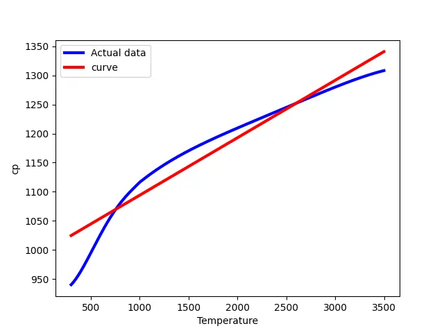
figure. actual data verses linear curve fit
By using the cubic polynomial it has a minor difference in the plot so it
does not has a lot of variation in the points so it can be used as a governing
equation.
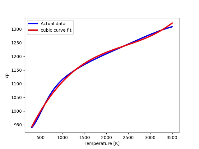
figure. actual data verses cubic curve fit
In this graph we follow same procedure but polynomial order we take fourth. Then
we got perfect plot.
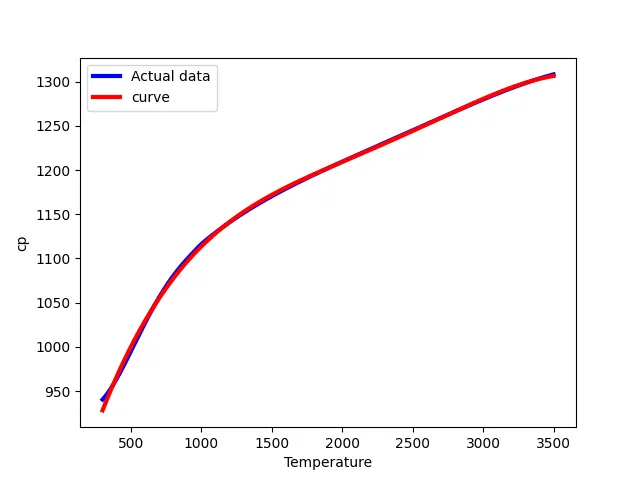
figure. perfect curve fit
CONCLUSION:-
In this graph we can get perfect fit when polynomial order increases
then we got perfect fit.