Project 2 - Rankine cycle Simulator
RANKINE CYCLE SIMULATOR
The Rankine cycle or Rankine Vapor cycle is the process widely used by power plants such as
coal-fired power plants or nuclear reactors. In this mechanism, a fuel is used to produce heat within
a boiler, converting water into steam which then expandas though a turbine producing useful work.
This process was developed in 1859 by Scottish engineer William J.M. Rankine. This is a thermodynamics
cycle which converts heat into mechanical energy-which usually gets transformed into elctricity by
electrical generation.
RANKINE CYCLE COMPONENTS:-
The four basic components of Rankine cycle are shown in figure each components in the cycle is regarded
as control volume, operating at steady state.
Pump:- The liquid condensate leaving the condenser at the state 1 is pumped to the operating pressure
of the boiler. The pump operation is considered isentropic.
Boiler:- The vapor leaving the boiler enters the turbine, where it expands isentropically to the condenser
pressure at the state 4. The work produced by the turbine is rotary (shaft) work and is used to drive an
electric generator or machine.
Condenser:- The condenser is attached at the exit of the turbine. The vapor leaving the turbine is wet vapor
and it is condensed completely in the condenser to the state 1, by giving its latest heat to some other cooling
fluid like water.
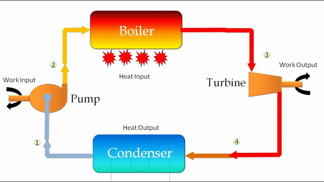
Figure. Rankine Cycle
The efficiency of the Rankine cycle is limited by the high heat of vaporization by the fluid. The fluid must be cycled
through and reused constantly, therefore water is the most practical fluid for this cycle. This is not why many power
plants are located near a body of water-that's for waste heat.
Applying the steady flow energy equation (SFEE) to all the process, neglecting the friction losses and change in
kinetic and potential energy.
for Boiler :- Q1=h1-h4
for Turbine :- Wt=h1-h2
for Condenser:- Q2=h2-h3
for Pump:- Wp= h4-h3
The capacity of the steam plant is often expressed interms of Steam Rate (SR) or Specific Steam Consumption (SSC)
S.S.C= 3600/Wn in Kg/kWh.
MAIN CODE:
clear all
close all
clc
% Displaying
disp('RANKINE CYCLE');
disp('1-2 is Isentropic Expansion in the turbine');
disp('2-3 is constant pressure heat removal in the condenser');
disp('3-4 is Isentropic compression in the pump');
dips('4-1 is constant pressure heat addition in the boiler');
% Obtaining the input data
p1=input('nValue of pressure at turbine inlet, p1(in bar)= ');
T1=input('nValue of temperature at turbine inlet, T1(in degree.C)= ');
p2=input('nValue of temperature at condenser inlet, p2(in bar)= ');
% Extracting data defining variables
% State point 1
h1=XSteam('h_pT',p1,T1);
s1=XSteam('s_pT',p1,T1);
% State point 2
s2=s1;
sf2=XSteam('sL_p',p2);
sg2=XSteam('sV_p',p2);
x2=(s2-sf2)/(sg2-sf2)
hf2=XSteam('hL_p',p2);
hg2=XSteam('hV_p',p2);
h2=hf2+(x2*(hg2-hf2));
% State point 3
p3=p2;
s3=XSteam('sL_p',p3);
h3=XSteam('hL_p',p3);
% State point 4
s4=s3;
p4=p1
% Work done by turbine
Wt=h1-h2;
% work done to the run pump
v3=XSteam('vL_p',p3);
Wp=v3*(p4-p3)*100;
h4=h3+Wp;
% net work done
Wnet= Wt-Wp;
% Heat into the system
Qin=h1-h4;
% Heat out of the system
Qout=h2-h3;
% Thermal efficiency
eff=(Wnet/Qin)*100;
% Specific steam consumption
Sp_S=(3600/Wnet);
% Specific temperature at the state points
T3=XSteam('Tsat_p',p3);
T2=T3;
Cp4=XSteam('Cp_ps',p4,s4);
Cv4=XSteam('Cv_ps',p4,s4);
k=Cp4/Cv4;
T4=T3/(p3/p4)^((k-1)/K));
% Calculating the temperature, entropy and enthalpy at the vapor and liquid
% line for plotting
T6=XSteam('Tsat_p',p1);
s5=XSteam('sL_p',p1);
s6=XSteam('sV_p',p1);
h5=XSteam('hL_p',p1);
h6=XSteam('hV_p',p1);
T5=T6;
% Plotting the saturation curve
T=linspace(1,375,1000);
for i=1:length(T)
sf(i)=XSteam('sL_T',T(i));
sg(i)=XSteam('sV_T',T(i));
hf(i)=XSteam('hL_T',T(i));
hg(i)=XSteam('hV_T',T(i));
end
% Plotting T-s diagram
figure(1)
hold on
plot(sf, T, 'r', 'linewidth', 1)
plot(sg, T, 'r', 'linewidth', 1)
plot([s1 s2],[T1 T2], 'k', 'linewidth',2)
plot([s2 s3],[T2 T3], 'k', 'linewidth',2)
plot([s3 s4],[T3 T4], 'k', 'linewidth',2)
plot([s4 s5],[T4 T5], 'k', 'linewidth',2)
plot([s5 s6],[T5 T6], 'k', 'linewidth',2)
sc1=linspace(s6,s1,1000);
for i= 1:length(sc1)
Tc1(l)=XSteam('T_ps',p1, sc1(l));
end
plot(sc1, Tc1, 'k', 'linewidth',2)
text(s1+0.1, T1, '1')
text(s2+0.1, T2, '2')
text(s3, T3-20, '3')
text(s4, T4+20, '4')
title('Temp vs Entropy plot')
xlabel('Entropy, s (KJ/kgk')
ylabel('Temperature (degree C')
legend('Saturation curve')
% Plotting h-s diagram
figure(2)
hold on
plot(sf, hf, 'r', 'linewidth', 1)
plot(sg, hg, 'r', 'linewidth', 1)
plot([s1 s2],[h1 h2], 'k', 'linewidth',2)
plot([s2 s3],[h2 h3], 'k', 'linewidth',2)
plot([s3 s4],[h3 h4], 'k', 'linewidth',2)
hc=linspace(h4,h5,100);
for k= 1:length(hc)
sch(k)=XSteam('s_ph',p1, hc(k));
end
plot(sch, hc, 'k', 'linewidth',2)
plot([s5 s6],[h5 h6],'k', 'linewidth', 2)
for m=1:length(sc1)
hc1(m)=XSteam('h_ps',p1,sc1(m));
end
text(s1+0.1, h1, '1')
text(s2+0.1, h2, '2')
text(s3, h3-100, '3')
text(s4, h4+200, '4')
title('Enthalpy vs Entropy plot')
xlabel('Entropy, S(KJ/kgk')
ylabel('Enthalpy, H(KJ/kgk')
legend('Saturation curve', 'location', 'northwest')
% Displaying Results
disp('RESULTS');
fprintf('\n At state point 1:n');
fprintf('\n p1: %8.3f barn', p1);
fprintf('\nT1: %8.3f Cn', T1);
fprintf('\n h1: %8.3f KJ/Kgn', h1);
fprinf('\n s1: %8.3f KJ/Kgnn', s1);
fprintf('\n At state point 2:n');
fprintf('\n p2: %8.3f barn', p2);
fprintf('\n T2: %8.3f Cn', T2);
fprintf('\n h2: %8.3f KJ/Kgn', h2);
fprinf('\n s2: %8.3f KJ/Kgknn',s2);
fprintf('\n x2: %8.3fnn', x2);
fprintf('\n At state point 3:n');
fprintf('\n p3: %8.3f barn', p3);
fprintf('\n T3: %8.3f Cn', T3);
fprintf('\n h3: %8.3f KJ/Kgn', h3);
fprinf('\n s3: %8.3f KJ/Kgnn', s3);
fprintf('\n At state point 4:n');
fprintf('\n p4: %8.3f barn', p4);
fprintf('\n T4: %8.3f Cn', T4);
fprintf('\n h4: %8.3f KJ/Kgn', h4);
fprinf('\n s4: %8.3f KJ/Kgnn', s4);
fprintf('\n Turbine Work: %8.3f KJ/Kgn', Wt);
fprintf('\n Pump Work: %8.3f KJ/Kgn', Wp);
fprintf('\n Wnet: %8.3f KJ/Kgn', Wnet);
fprintf('\n Efficiency: %8.3f Percentn', eff);
fprintf('\n Sp. Steam Consumption: %8.3f in KJ/KWn', Sp_S);
EXPLANATION:-
We start program before write clear all, close all and clc.
clear all:- Deleted all current workspace from system memory.
close all:- Deleted all images.
clc:- Clear the command window.
The creation of Rankine cycle simulator starts with some input value which are required to
calculate the other state point in cycle eventually.
The Rankine cycle process is displayed in the command window and then inputs are entered which are inlet pressure for
turbine, temperature at turbine inlet and pressure at condenser.
Then we are using XSteam function file for reading state point. First we get the value of enthalpy and entropy at state point 1 from
the XSteam function file.
As process from 1-2 is isentropic compression the entropy at point 1 is equal to point 2. The term (s_pT, p1, T1) refers to entropy at
pressure and temperature point 1.
The term 'sg' and 'sf' are referred to saturated liquid and saturated vapor entropy respectively. This value is used to calculate other function
according to mathematical relations.
Similarly, other points are taken from XSteam function file which are necessary to calculate other parameters. After that work done in
turbine and pump are calculated for further getting the net work done Rankine cycle.
After calculating the net work done the efficiency of the Rankine cycle is calculated along with specific steam consumption which is steam
consumed by a locomotive cylinders per unit of output ofwork done.
Then temperature at each point of cycle is calculated using input taken from start of the program and data taken from XSteam file. Temperature
range is defined using linspace command For giventemperature range from lower to higher entropy points are calculated to create the T-S plot.
Similarly, another for loop is used to create the saturation curve in each plot.
Then plotting is done respectively for T-S and H-S graph in Rankine cycle and each state point value has been put in command window.
Results of the cycle simulation is displayed over command windows using fprintf command.
OUTPUT:-
To make the graph more delibrated we are changing some value in the inputs by increasing the inlet pressure and temperature along with
condenser pressure also which results in following graphs.
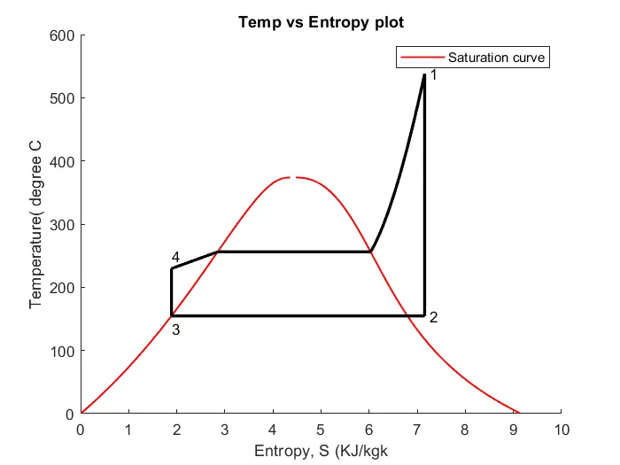
From the above diagram as we can see along the saturation curve point 1 start with turbine from which heat rejection is started which is again
isentropic process. The steam is get cooled in condenser and in form of saturated liquid as it is under the curve. The it was pumped to enter in boiler
where its temperature is increased to change it from saturated liquid to saturated vapor form.
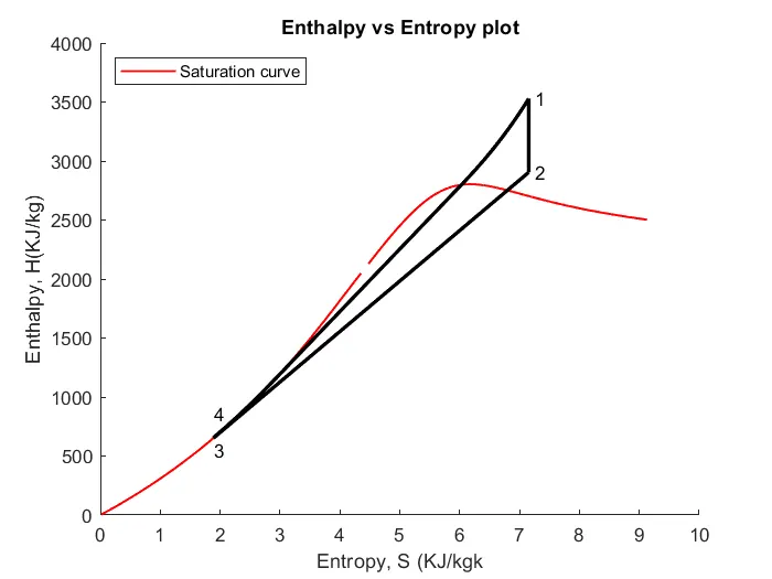
As we can see from above plot the steam entropy changes during the process with respect to enthalpy. As the heat added in the system the entropy
has been increased and similarly as the heat removed from the system the entropy drops with similar rates.
The values for the state point in command windows are given as:-
For the Inlet pressure in Turbine as= 44 bar
Inlet temperature in Turbine= 538 degree cel
Pressure in condenser= 5.38 bar
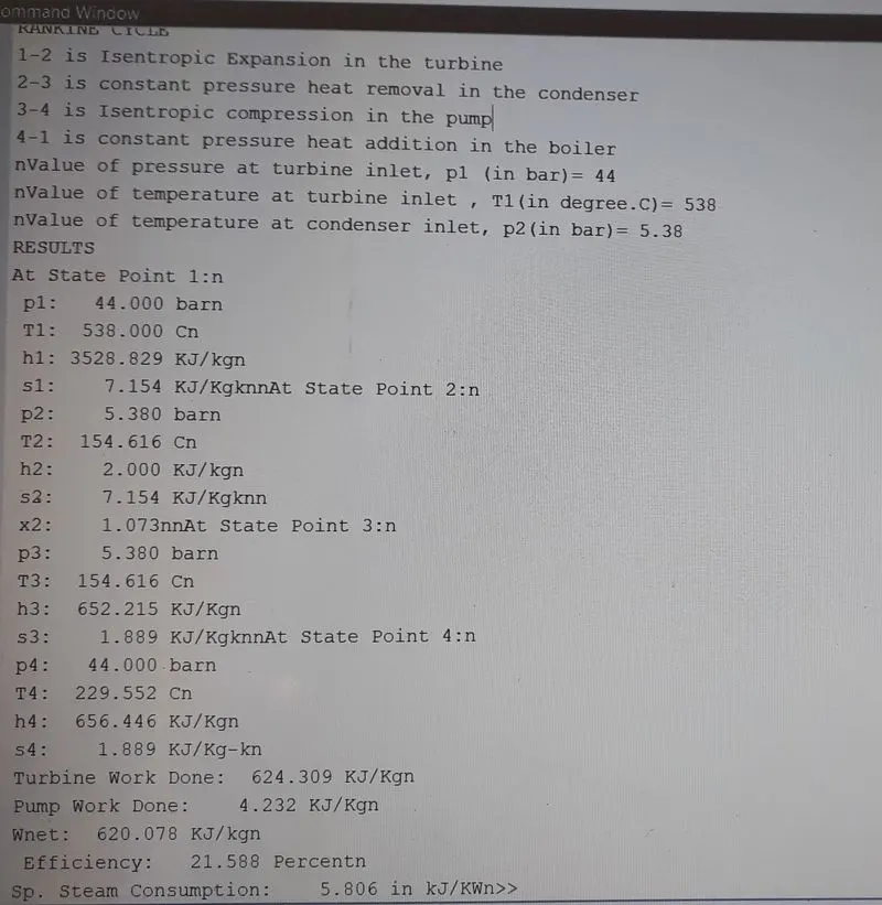
For the parameters given in the challenge the graph will look like this:-
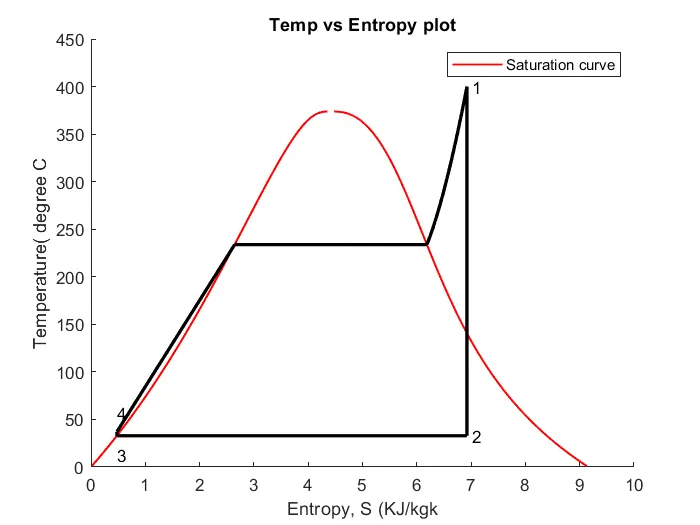
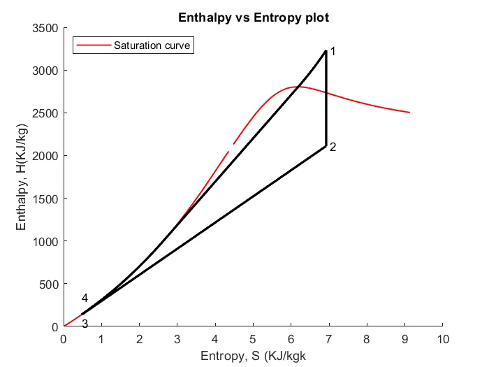
For Input given in challenging:-
For Inlet pressure in Turbine as= 30 bar
Inlet Temperature in Turbine= 400 deg. Cel
Pressure in Condenser= 0.05 bar
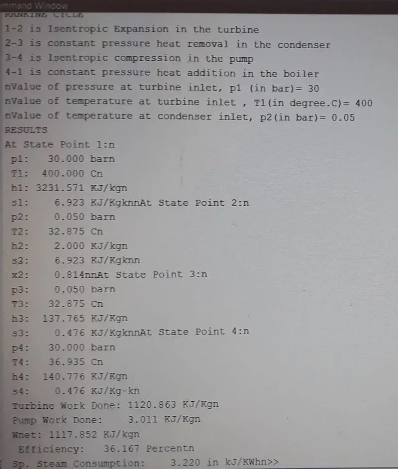
From the two different input values it is seen that increasing the pressure and temperature in turbine
result in lowering the efficiency of Rankine cycle.
specific steam consumption is 3.220 in KJ/KWh.
ERROR:-
while programing that time i accidentilly type XStem instead of XSteam.
Then MATLAB alert me,
Unrecognized function or variable 'XStem'.
Error in rankine_cycle (line 44)
v3= XStem('vL_p',p3);
Then i corrected my mistke. I typed XSteam then i got result.
CONCLUSION:-
So, we have created the Rankine cycle simulator for the given input, in which we have taken the data from
XSteam function file.