Week 3 - Solving second order ODEs

To solve a Second order Ordinary Differential Equation

In Engineering, ODE is used to describe the transient behavior of a system. A second order ordinary differential equation is an ordinary differential equation in which any derivatives

with respect to the independent variable have order no greater than 2.

Ordinary differential equations helps us to solve the many engineering systems. Such as harmonic motions, vibrations, damping,etc.

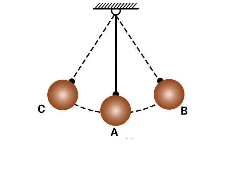
figure. Simple pendulum

In this figure one ball is fixed at wire end and one end of wire fixed at a pivot. This pendulum swing point B to point C. when the pendulum swing with wire, that time pendulum create a angle 'theta'.

A simple pendulum consist of a mass 'm' hanging from a string of length 'l' and fixed at a pivot point. When displaced to an initial angle 'theta' and released, the pendulum will swing back

fourth with periodic motion.

The equation is given by,

In the above equation,

g = gravity in m/s2,

L = length of the pendulum in m,

m = mass of the ball in kg,

b=damping coefficient.

Inputs are given in the problem,

L=1 metre,

m=1 kg,

b=0.05.

g=9.81 m/s2.

And Initial conditions are also given,

Angular displacement=0,

Angular velocity= 3 rad/sec, at time=0

The motion is simulated between 0-20 sec.

% function program for solving second order ode

function [dtheta_dt]= challenging_ode_func(t,theta,b,g,l,m);

theta1=theta(1);

theta2=theta(2);

dtheta1_dt=theta2

dtheta2_dt=-(b/m)*theta2-(g/l)*sin(theta1);

dtheta_dt=[dtheta1_dt; dtheta2_dt]

end

MAIN CODE:-

clear all

close all

clc

% Inputs

b= 0.05;

g= 9.81;

l= 1;

m=1;

% Initial condition

theta_0=[0;3];

% time points

t_span=linspace(0,20,30);

% Solve ode

[t_results]= ode45(@(t,theta) chalenging_ode_func(t,theta,b,g,l,m), t_span,theta_0);

% Plotting

figure(1)

plot(t,results(:,1))

hold on

plot(t,results(:,2))

xlabel('time')

ylabel('Velocity(Red) & Displacement(Blue)')

holf off

% Animation of the simple pendulum

figure(2)

ct=1;

for i=1:length(results(:,1))

x0=0;

y0=0;

x1=l*sin(results(i,1));

y1=-l*cos(reults(i,1));

% for surface line

plot([-1 1],[0 0],'linewidth',3,'color','b');

hold on

% for point of contact of wire and surface

plot([0 0],[0 0],'o','Markersize',10,'markerfacecolor','r')

hold on

% for wire representation

plot([x0 x1],[yo y1],'linewidth',2,'color','g')

hold on

% for bob represntation

plot(x1,y1,'o','Markersize',30,'markercecolor','r')

axis([-1.5 1.5 -1.5 0.5])

hold on

pause(0.0001)

M(ct)=getframe(gcf)

hold off

ct=ct+1

end

% Making the animation of the simple pendulum

movie(M)

videofile=VideoWriter('challenging_ode.AVI')

open(videofile)

writeVideo(videofile,M)

close(videofile)

EXPLANATION:-

we start program before write clear all, close all and clc.

clear all- Clear the workspace.

close all- Deleted the all figure and graphs that' exists.

clc- Clear the all window command.

The inputs of simple pendulum are given,

Gravity(g)=9.81 in m/s2, Length of the pendulum(l)=1 in m, Mass of the ball(m)=1 in kg, Damping coefficient=0.05.

t_span- t_span is a coomand which is used to ode45 solver which then specifies the time span of the iterations that is solving the ordinary differential equation.

ode45- It is a function of MATLAB that solves the ordinary and partial differential equation using a numerical method. In this problem the higher order is 2. So we have to take the

two constant values then tha equation is changed to simple differential equation.

The function should take at least two inputs to solve the equation to the approximate results. The ode 45 function has syntax which is we need to specify the 't' and ' theta' and the

output may be of 't','theta' and the inputs(b,g,l,m).

The syntax of ode45 solver is,

[t_results]= ode45(@(t,theta) chalenging_ode_func(t,theta,b,g,l,m), t_span,theta_0);

Then we used plotting command, we got images of time verses angular velocity and anguar displacement. In this figure i gave name of xlabel and ylabel.

After we used animation command, in this command we take ct. ct is the count a each and every position of pendulum bob and then store the data.

In this animation command we used for loop command whichb is used create specified set of points to keep the bob at different position.

Then x0 and y0 take 0 values because this values take for the fixed the point at the one end of wire. And x1 ,y1 values are fixed point to the another different position of the bob.

Then we gave 'Marker' command for the bob size ane bob face colour.

At the end of for loop we set of positions for each and every points.

movie(M):- Which is used to create a film and stored the data of the motion of the pendulum.

videoWriter:-This command specifies the name of the file and type of data stored in it.

open:-This command is used to open the file where the video is storing the file.

WriteVideo:-This command which is used to creat the video animation by using M file.

colse:-This command which is used to the close the videon file.

OUTPUTS:-

A plot is drawn between the angular velocity and angular displacement of the motion of simple pendulum.

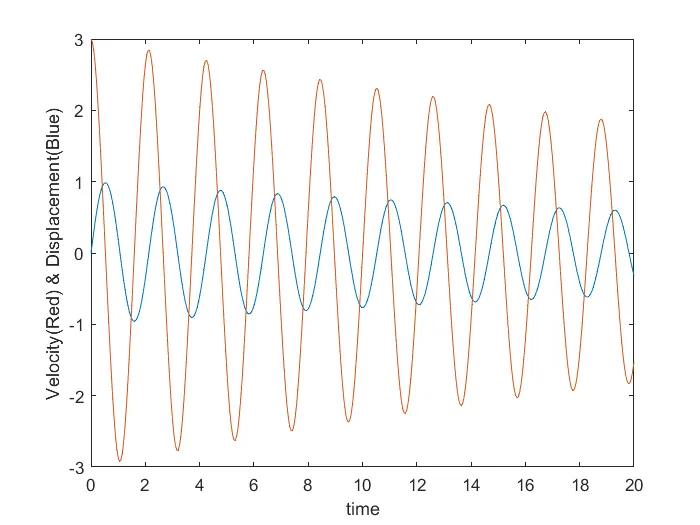
figure. angular velocity and angular displacement verses time

The blue curve is the angular displacement which is starts from zero. And red curve is the angular velocity is starting from 3(rad/sec). At the end of the t_span both angular

displacement and angular velocitybecomes zero and the motion of simple pendulum becomes zero which is become rest. Angular displacement and angular velocity is decreasing

by the incresed time this is due to the introduction of damper. It means that damping coefficient which absorbs the vibrations to make the body in equillibrum position.

ERROR FACED WHILE PROGRAMMING:-

I tyep in program by mistake 'writevideo' instead of 'writeVideo', then matlab gave me alert,

Unrecognized function or variable 'writevideo'.

Error in challenging_ode (line 63)

writevideo (videofile,M);

Then i corrected my mistake, i wrote in program 'writeVideo'.

Animated File:-