Project 1 - Parsing NASA thermodynamic data
To write a code in MATLAB to parse nasa thermodynamics data file and then calculate thermodynamics properties of
various gas species.
OBJECTIVE:-
Write a function that extracts the 14 co-efficients and calculates the enthalpy, entropy and specific heats for all the
species in the data file. You will be reading this file.
Calculating the molecular weight of each species.
Plotting the specific heat, enthalpy and entropy for the local temperature range.
Saving the plots as images with appropriate names and dumping folders for each species.
FILE PARSING:-
File parsing is a string or symbol either in natural language computer language or data structure conferming to the
rules of the former grammer.
MATHEMATICAL EQUATIONS:-
For Specific Heat
cp=(a1+a2.*T+a3.*T.2+a4.*T.3+a5.*T.4)*R;
For Enthalpy
H=(a1+(a2.*T)/2)+(a3.*T2)/3+(a4.*T.3)/4+(a5.*T4)/5+(a6./T))*R.*T;
For Entropy
S=a1.*log(T)+a2.*T+(a3.*T.2)/2+(a4.*T.3)/3+(a5.*T.4)/4+a7;
MAIN CODE:-
clear all
close all
clc
% Getting the data file
f1=fopen('THERMO(1).dat','r')
fgetl(f1)
A=strsplit(fgetl(f1).' ');
% Reading the global temperature range
global_low_temp=str2num(A{2});
global_mid_temp=str2num(A{3});
global_high_temp=str2num(A{4});
% Skipping next three lines
for i= 1:3
fgetl(f1)
end
% Reading the species
for i= 1:53
header=fgetl(f1)
speciesheader=strsplit(header,' ')
species_name=speciesheader{1}
t1=str2double(speciesheader{end-3})
t2=str2double(speciesheader{end-2})
t3=str2double(speciesheader{end-1})
% Getting the first line coefficients (a1-a5)
line_1=fgetl(f1)
a=strfind(line_1,'E')
a1=str2double(line_1(1:a(1)+3));
a2=str2double(line_1(a(1)+4:a(2)+3))
a3=str2double(line_1(a(2)+4:a(3)+3))
a4=str2double(line_1(a(3)+4:a(4)+3))
a5=str2double(line_1(a(4)+4:a(5)+3))
% Getting second line coefficients(a6-a10)
line_2=fgetl(f1)
a_1=strfind(line_2,'E')
a6=str2double(line_2(1:a_1(1)+3))
a7=str2double(line_2(a_1(1)+4:a_1(2)+3))
a8=str2double(line_2(a_1(2)+4:a_1(3)+3))
a9=str2double(line_2(a_1(3)+4:a_1(4)+3))
a10=str2double(line_2(a_1(4)+4:a_1(5)+3))
% Getting third line coefficients (a10-a14)
line_3=fgetl(f1)
a_2=strfind(line_3,'E')
a11=str2double(line_3(1:a_2(1)+3))
a12=str2double(line_3(a_2(1)+4:a_1(2)+3))
a13=str2double(line_3(a_2(2)+4:a_1(3)+3))
a14=str2double(line_3(a_2(3)+4:a_1(4)+3))
% Making the Directory
mkdir(['C:\Desktop\matlab\file\images\',species_name]);
T=linspace(t1,t2,1000);
R=8.314;
% To getting array of specific heat, enthalpy, entropy
for k=1:length(T)
% To compare the species temperature to assign the coefficients
% a1-a7(high temperature coefficients), a8-a14(low temperature coefficients)
if T(k)>t3
% high temperature coefficients
cp(k)=(a1+a2.*T(k).^2+a3.*T(k).^2+a4.*T(k).^3+a5.*T(k).^4)*R;
H(k)=(a1+(a2.*T(k))/2+(a3.*T(k).^2)/3+(a4.*T(k).^3)/4+(a5.*T(k)^4)/5+(a6./T(k)))*R.*T(k);
S(k)=a1.*log(T(k))+a2.*T(k)+(a3.*T(k).^2)/2+(a4.*T(k).^3)/3+(a5.*T(k).^4)/4+a7;
% low temperature coefficients
cp(k)=(a8+a9.*T(k).^2+a10.*T(k)^2+a11.*T(k).^3+a12.*T(k).^4)*R;
H(k)=(a8+(a9.*T(k))/2+(a10.*T(k).^2)/3+(a11.*T(k).^3)/4+(a12.*T(k).^4)/5+(a13./T(k)))*R.*T;
S(k)=a8.*log(T(k))+a9.*T(k)+(a10.*T(k).^2)/2+(a11.*T(k).^3)/3+(a12.*T(k).^4)/4+a14;
end
end
% Plotting the graphs
figure(1)
plot(T,cp)
grid on
title(species_name)
xlabel('Temperature')
ylabel('Specific Heat')
figure(2)
plot(T,H)
grid on
title(species_name)
xlabel('Temperature')
ylabel('Enthalpy')
figure(3)
plot(T,S)
grid on
title(species_name)
xlabel('Temperature')
ylabel('Entropy')
% Changing the directory and saving the file
saving=(['C:\Desktop\matlab\file\images\',species_name]);
cd(saving)
saveas(1,'Specific Heat','jpg');
saveas(2,'Enthalpy','jpg');
saveas(1,'Entropy','jpg');
%cd=('C:\Desktop\matlab\file\programs');
% molecular_mass_calculations
species=species_name
elements=['H','C','O','N','A'];
atomic_weight=[1.0079 12.0107 15.0999 14.0067 39.948];
mol_mass=0;
for i= 1:length(species)
for j= 1:length(elements)
if strcmpi(species(i),elements(j))
mol_mass=mol_mass+atomic_weight(j);
position=j;
end
end
end
n=str2double(species(i))
if n>1
mol_mass=mol_mass+elements(position)*(n-1);
end
disp(sprintf('Molecular Weight of %s:%f u',species,mol_mass))
end
fclose(f1)
EXPLANTION:-
Starting program before type clear all, close all and clc.
clear all- Delete the workspace.
close all- Delete the all images.
clc- Clear the command history.
we used "(fopen)" command. By this command we will open the file with its specific name which is
'THERMO(1).dat' format and 'r' indicates the read that file. It means we have a file with some name
and we want to open that file in our matlab software to read that data for some changes or for other
additional help then this all will be done by fopen command and with 'r' symbol coding natation. If
we want to create any file then we will use 'w' symbol coding notation which refers 'w' to write.
After that we used "fgetl(f1)" command for taking the line. This command fgetl(f1) means taking line
from f1 file. Once again typing code of fgetl(f1) refers taking second line from file f1. So similarly we can
use this command so many times as same as the number of lines to take from files in sequence. So in our
coding first five lines are header related line l1 to l5 which are not generally our area of focus.
After that we used "strsplit" command refers to the string split and ' ' is a string spliter. It means here is that
the line l6 which is in string format will be splitted by strsplit command and this whole splitting or cutting of string
will occure where string splitter will be present which is a space in string line and which is represented in coding
by ' '. These splitted part are stored in A varaible element.
Then we used "findstr" command for refers to the find string at particular location in our case is at point which
represent in our coding by , ' ' . It helps to selecting temperature range string and then after that with the help
of strsplit we will find different temperature string which are stored in 'temperature' name elements.
In this program we will split the line by string splitter 'E'. So by this way we will split 14 coefficients. a1-a7 which are high
temperature coefficients and a8-a14 which are low temperature coefficients.
After that we used str2double and str2num command. This two commands are same . This command is converts the text in
str to double precision values.str contains text that represents real or complex numeric values. str can be a character vector,
a cell array of character vectors.
Then we used "mkdir" command to storing the plots for species_name, we will make directory by "mkdir" command is
mkdir(['C:\Desktop\matlab\file\images\',species_name]).
C is disc name presented in laptop , This file is present in desktop and matlab folder. file is a folder present under disc C and
species_name is also folder under file folder but it is automatically generated by command and species_name are variable folders
name.
There are three categories of plots for each species. First is plotting between Temperature and Specific Heat. Second is plotting
between Temperature and Enthalpy and Third is plotting between Temperature and Entropy.
After that we used "cd" for refers to change directory. To save the plots in different directory or disc therefore we are doing change
of current directory to change directory path.
Now we will code for calculating molecular weight for each species with the help of creating function which is,
species=species_name .
Under this function the basic idea behind to calculating the molecular weight is that firstly we will match the molecule atoms one by
one to the atoms present in our function which are, elements=['H','C','O','N','A'], with the help of strcmpi command which refers to string
comparision. Then with matched atom we will take atom-weight and add , correspondingly to matched atom. The coding in our program
is like that mol_mass=mol_mass+atomic_weight(j);
After that we used str2double command for used to calculation of molecular weight. The coding in our program is like that
mol_mass=mol_mass+elements(position)*(n-1).
Here we are taking (n-1) in multiply instead of n beacause we are input second time coding, mol_mass=mol_mass+elements(position)*(n-1).
So by this two times, the effect be double additional so to balance this we are reducing n to n-1 time.
After that we used "fclose(f1)" command is for closing the f1 file.
OUTPUTS:-
SCREENSHOT OF DIRECTORY:-
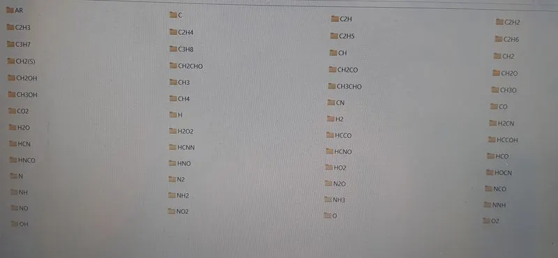
figure(1). screenshot of directoy
PLOT FOR O2
Specific Heat:-
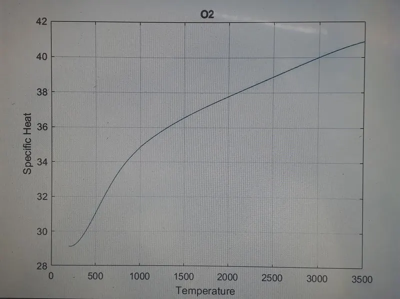
figure(2). specific heat verses temperature for O2
Enthalpy:-
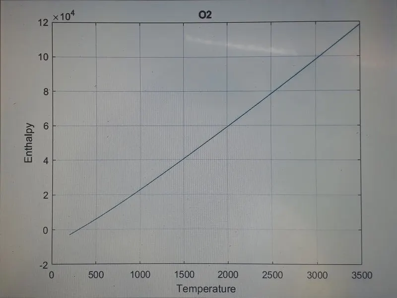
figure(3). enthalpy verses temperature for O2
Entropy:-
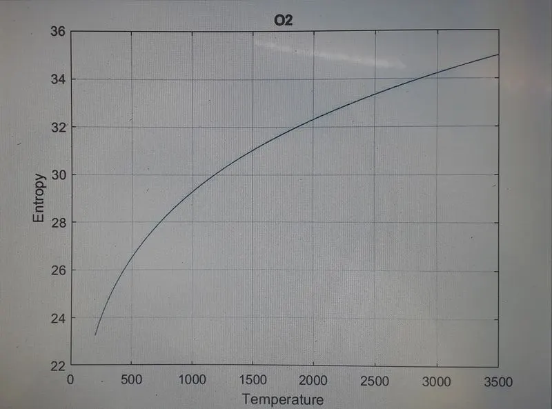
figure(4). entropy verses temperature for O2
PLOT FOR N2
SPECIFIC HEAT:-
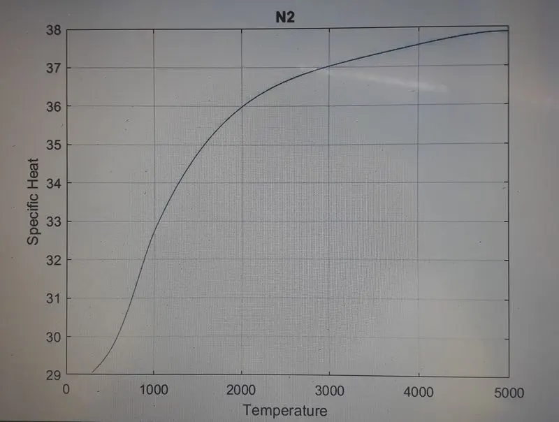
figure(5). specific heat verses temperature for N2
ENTHALPY:-
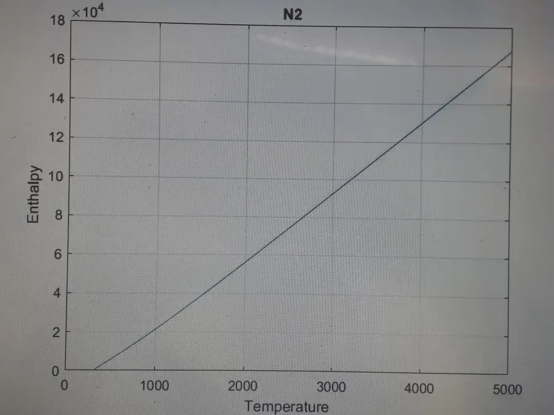
figure(6). enthalpy verses temperature for N2
ENTROPY:-
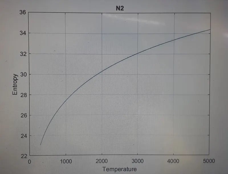
figure(7). entropy verses temperature for N2
PLOT FOR CO2
SPECIFIC HEAT:-
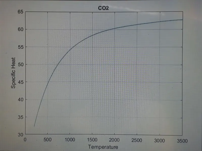
figure(8). specific heat verses temperature for CO2
ENTHALPY:-
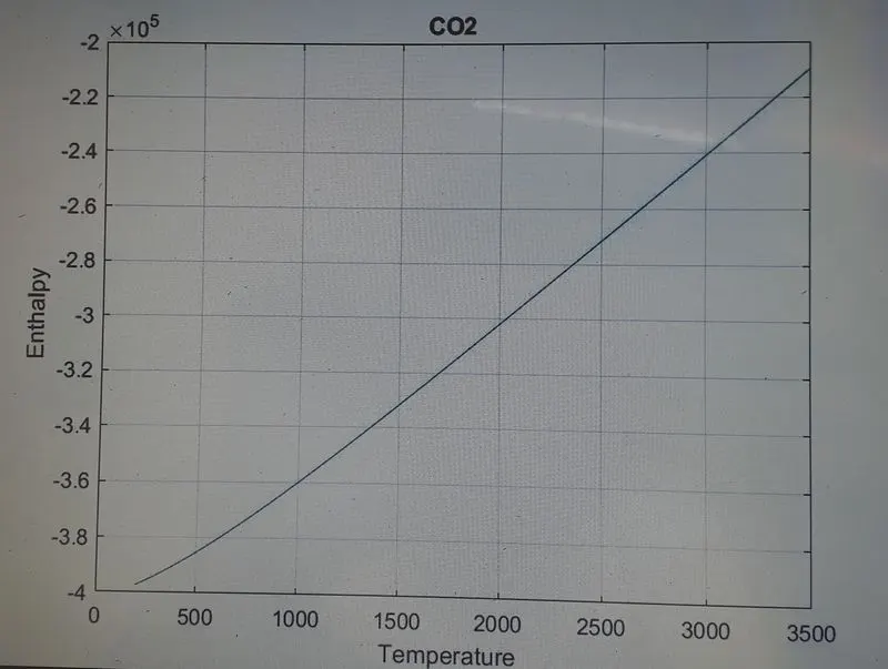
figure(9). enthalpy verses temperature for N2
ENTROPY:-
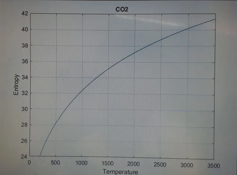
figure.(10) entropy verses temperature for N2
CONCLUSION:-
Hence all the properties for various elements are plotted to know their variation with temperature.
ERROR:-
While programing i gave all the temperature name in program T(k) but all specific heat, enthalpy and entropy not gave T(k).
example. cp(k), H(k), S(k).
when i will not use that time i don't gave all plots.
when i used cp(k), H(k) and S(k) that time i got all plot images.