Week 4.1 - Genetic Algorithm
To write a code in MATLAB to optimise the stalagmite function and find the global maxima of the function.
OPTIMIZATION:- Optimization is the process of making something as fully perfect, functional, or effective as possible.
Optimization refers to the finding the values of inputs in such a way that we get the 'best' output values. This optimization is refers
to maximizing and minimizing one or more objective functions, by varying the input parameter.
The set of all possible solutions or values which is the inputs can take make up the search space. In this search
space, lies a point or a set of points which gives the optimal solution. The aim of optimization is to find that point or
set of points in the search space.
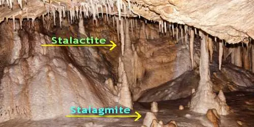
STALAGMITE:- A stalagmite is an upward-growing mound of mineral deposits that have precipitated from water dripping onto the floor of
a cave. Most stalagmites have rounded or flattened tips. There are many other types of mineral formations found in caves.
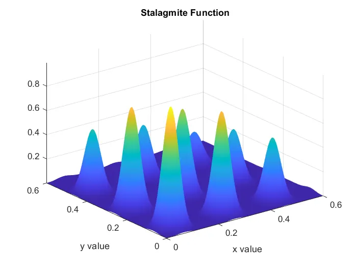
A stalagmite function generally refers to the function which we are generating values over a stalagmite kind of surface for finding
out the local and global maxima and minima of that particular given function.
For this in MATLAB we are using a method called 'Optimization'. It is a programming which does a selection of the best element with regard
to some criterion from set of population.
Optimization is done by systematically choosing input values from within an allowed set and computing the results of the function.
In matlab to perform to perform optimization we use 'Genetic Algorithm' method which is a inbuild function in matlab to find the global
maxima of that given stalagmite function.
GENETIC ALGORITHM:- A Genetic Algorithm is a search experimental that is simulated by Charles Darwin's theory of natural evolution.
This algorithm reproduces the process of natural selection where the appropriate individuals are selected for reproduction in order to produce
offspring of the next generation.
The genetic algorithm is a technique for solving both constrained and unconstrained optimization problem that are based on natural selection, the
process that drives biological evolution. The genetic algorithm constantly modifies the population size of individual solutions.
Types of genetic Algorithm:-
1) Initialization of Population (Coding):-
The codes generates its random population of defined size andfrom that population the code evaluates the fitness of the member of the population
according to which it forms new population based on no. of iterations performed.
2) Fitness Function:-
It is the function which is we have to optimize and its optimization is done with the help of number of generation which have been formed by the code accordance
with the fitness value of each member generated, these fitness value are used for the reproduction of the children.
3) Selection:-
The idea of the selection phase is to select the fittest individuals and let them pass their genes to the next generation. The main goal of this phase is to find the
region where the chance of getting the best solution are more.
Inspiration for this is form of the survival of the fittest.
It should be a balance between exploration and exploitation of search space.
Genetic algorithm tries to move the genotype to higher fitness in the search space.
Too strong fitness selection bias can lead to sub-optimal solutions.
Too little fitness bias selection results in unfocused search.
4) Reproduction:-
Generation of offspring happen in two ways
a) Crossover
b) Mutation
a) Crossover:-
Crossover is the most significant stage in the genetic algorithm. During crossover, a random point is selected while mating a pair of parents to generate offspring.
There are three major types of crossover.
Single Point Crossover:- A point on both parent's chromosomes is picked randomely, and designated a 'crossover point'.
Two-Point Crossover:- Two crossover points are picked randomly from the parent chromosomes.
Uniform Crossover:- In a uniform crossover, typically, each bit is chosen from either parent with equal probability. The new offspring are added to the population.
b) Mutation:- In a few new offspring formed, some of their genes can be subjected to a mutation with low random probability. This indicates that some of the bits
in the bit chromosome can be flipped. Mutation happens to take care of diversity among the population and stop premature convergence.
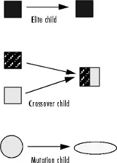
Then it is said that the genetic algorithm has provided a set of solution to our problem. The poulation has a fixed size. A new generation are formed, individuals with
least fitness die, providing space for new offspring. The sequence of phases is repeated to produce individuals in each new generation which are better than the previous
generation.
ADVANTAGES OF GA:-
1) It Does not require any derivative information.
2) It is a faster and more efficient as compared to the traditional methods.
3) It has very good parallel capabilities.
4) Optimizes both continuous and discrete functions and also muitiobjective problems.
4) Provides a list of good solutions and not just a single solution.
5) Useful when the search space is very large and there are a large number of parameters involved.
LIMITATIONS OF GA:-
1) Genetic algorithm are not suited for all problems, especially problems which are simple and for which derivative information is available.
2) Fitness value is calculated repeatedly which might be computationally expensive for some problems.
3) Being stochastic, there are no guarantees on the optimality or the quality of the solution.
4) If not implemented properly, the GA may not converge to the optimal solution.
APPLICATIONS OF GA:-
1) Optimization:- Genetic algorithms are most commonly used in optimization problems where in we have to maximize or minimize a given objective function value under a given
set of contraints. The approach to solve optimization problems has been highlighted throughout the tutorial.
2) Economics:- GAs are also used to characterize various economic models like the cobweb model, game theory equilibrium resolution, asset pricing, etc.
3) Neural Network:- GAs are also used to train neural networks, particularly recurrent neural networks.
4) Image Processing:- GAs are used for various digital image processing(DIP) tasks as well like dense pixel matching.
5) Vehicle routing problems:- With multiple soft time windows, multiple depots and a heterogeneous fleet.
6) DNA Analysis:- GAs have been used to determine the structure of DNA using spectrometric data about the sample.
SYNTAX FOR GA:-
The format for writing genetic algorithm in matlab is below,
f_min=ga(@function, nvars, A, B, Aeq, Beq, LB, UB, nonlcon, intcon, options)
1) f_min is the local minima point.
2)@function is the function to be called.
3) nvars indicates the no. of variable used.
4) A and B are used to indicate any kind inequalities that exist in the function.
5) Same goes with Aeq and Beq.
6) LB= lower bound
7) UB= upper bound
8) nonclon gives a two vectors representing inequalities and equalities.
9) options is used to perform additional operations like increasing population size. This is done with the help of optimoptions.
FUNCTION CODE:-
function [f]=stalagmite(input_vector)
x= input_vector(1);
y= input_vector(2);
f1_x=(sin(5.1*pi*x+ 0.5)).^6;
f1_y=(sin(5.1*pi*y+ 0.5)).^6;
t1=((x-0.0667).^2)/(0.64);
f2_x=exp(-4.*log(2)*t1);
t2=((y-0.0667).^2)/(0.64);
f2_y=exp(-4.*log(2)*t2);
[f]=-(f1_x.*f2_x.*f1_y.*f2_y);
end
MAIN PROGRAM:-
clear all
close all
clc
x=linspace(0,0.6,150);
y=linspace(0,0.6,150);
num_cases=50
% Creating a 2D mesh
[xx yy]=meshgrid(x,y)
% Evaluating a stalagmite function
for i= 1:length(xx)
for j=1:length(yy)
input_vector(1)=xx(i,j)
input_vector(2)=yy(i,j)
f(i,j)=stalagmite(input_vector);
end
end
% Generating the surface
surfc(xx, yy, -f)
xlabel('x value')
ylabel('y value')
title('Stalagmite Function')
shading interp
MAIN CODE:-
clear all
close all
clc
x=linspace(0,0.6,150);
y=linspace(0,0.6,150);
num_cases=50
% Creating a 2D mesh
[xx yy]=meshgrid(x,y)
% Evaluating a stalagmite function
for i= 1:length(xx)
for j=1:length(yy)
input_vector(1)=xx(i,j)
input_vector(2)=yy(i,j)
f(i,j)=stalagmite(input_vector);
end
end
% Generating the surface
surfc(xx, yy, -f)
xlabel('x value')
ylabel('y value')
title('Stalagmite Function')
shading interp
% Study 1- Statistical behaviour
tic
for i=1:n
[inputs, fopt(i)]=ga(@stalagmite,2);
xopt(i)=inputs(1);
yopt(i)=inputs(2);
end
study1_time=toc
figure(1)
subplot(2,1,1)
hold on
surfc(xx, yy, -f)
shading interp
title('Unbounded inputs')
plot3(xopt, yopt, -fopt,'marker','o','markersize',5,'markerfacecolor','r')
subplot(2,1,2)
plot(-fopt)
xlabel('No. of Iterations')
ylabel('Function maximum')
% Study 2- Statistical behaviour with upper and lower bounds
tic
for i=1:n
[inputs, fopt(i)]=ga(@stalagmite,2,[],[],[],[],[0,0],[1,1]);
xopt(i)=inputs(1);
yopt(i)=inputs(2);
end
study2_time=toc
figure(2)
subplot(2,1 1)
hold on
surfc(xx, yy, -f)
shading interp
title('Statistical Behaviour with upper and lower bounds')
plot3(xopt, yopt, -fopt, 'marker','o','markersize',5,'markerfacecolor','r')
subplot(2,1,2)
plot(-fopt)
xlabel('Iterations')
ylabel('Function maximum')
% Study 3- Statistical behaviour with increaing iterations of GA
options=optimoptions('ga');
options=optimoptions(options,'PopulationSize',500);
tic
for i=1:n
[inputs, fopt(i)]=ga(@stalagmite,2,[],[],[],[],[0,0],[1,1],[],[],options);
xopt(i)=inputs(1);
yopt(i)=inputs(2);
end
study3_time=toc
figure(3)
subplot(2,1 1)
hold on
surfc(xx, yy, -f)
shading interp
title('Statistical Behaviour with increasing iterations')
plot3(xopt, yopt, -fopt, 'marker','o','markersize',5,'markerfacecolor','r')
subplot(2,1,2)
plot(-fopt)
xlabel('Iterations')
ylabel('Function maximum')
EXPLANATION:-
Start a program before type clear all, close all and clc.
clear all:- It is used to delete all workspace.
close all:- It is used to deleted the all plots.
clc:- It is used to clear all command windows.
The stalagmite function is defined separately. This function is later called into the main GA program.
Now we defined the x and y inputs using linspace commands.
Then input vectors are transformed into array [xx yy], so that it can be used to evaluate function of two variables and plotted three dimensional mesh.
Now the values in the different matrixs created can be put as an input into the function that we have created by calling it. By this we can get the value
of the stalagmite function at values of x and y.
Now since we have got the values of the function at various values, we now need to calculate the maxima value, which can be calculated using the ga
commands, which is an in built function in MATLAB.
Then, the total number of time the ga needs to run is defined 'n' values, and with help of for loop ga is made to run for each iteration and the value is
stored in an array.
GA generally gives the minima value (in built in MATLAB), but we need to maxima hence we can just inverse the stalagmite function by introducing a
'Negative Sign'.This Negative sign is inverse the stalagmite curve and the global maximas can be found instead of minima.
The total study time is calculated using the 'tic' and 'toc' command at the start and end of the ga for loop respectively.
The results are then plotted using the surfc command and plot command.
GA is made to run for three iterations, with each iteration having bounded inputs , unbounded inpts and increasing population size.
In a first study GA function runs for 50 iterations. Plots of the stalagmites and maximum values generated in each iteration .
In the second study GA function is incorporated with lower and upper bounds and runs for 50 iterations. Plots of the stalagmite and maximum values
generated in each iteration.
In the third study GA function is incorporated with lower and upper bounds along with the population size. And population size is took 500. Then plots of stalagmite and maximum values
generated in each iteration.
RESULTS:-
Study 1 Statistical Behaviour Unbounded:-
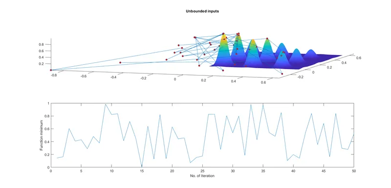
figure. Unbounded inputs and iteration
In this first study there are no lower and upper limit hence the GA does not the search space is between 0 and 1. It is clear that the results are
not that much accurate and giving a lot of variation in optimizing the function. first Study time is 2.59 seconds.
Study 2 Statistical behaviour with upper and lower bounds:-
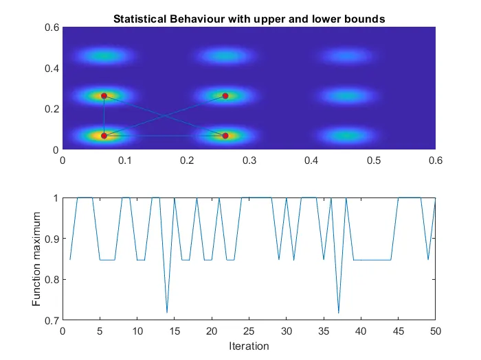
Figure. Statistical Behaviour with upper and lower bounds
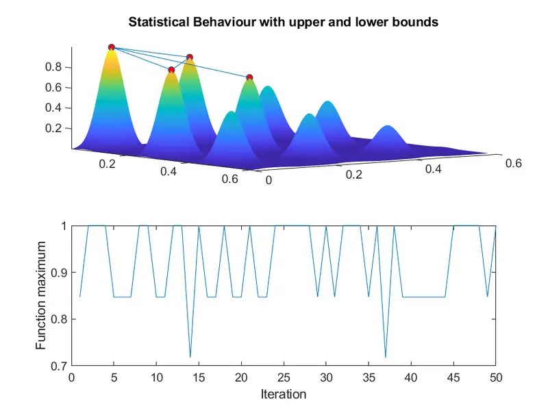
Figure. Statistical Behaviour with upper and lower bounds
In the second study lower and upper limits are included in the GA. Hence most of the maximum values obtained in each iteration varies
between 1 and 0.85. This method narrows down the maximum values to four points. It is clearly seen from tha above that after providing
the boundary limits the variation in the optimum value of the function has reduced.In that duration this second study time take 3.29 seconds.
Study 3 Statistical behaviour with increasing iterations:-
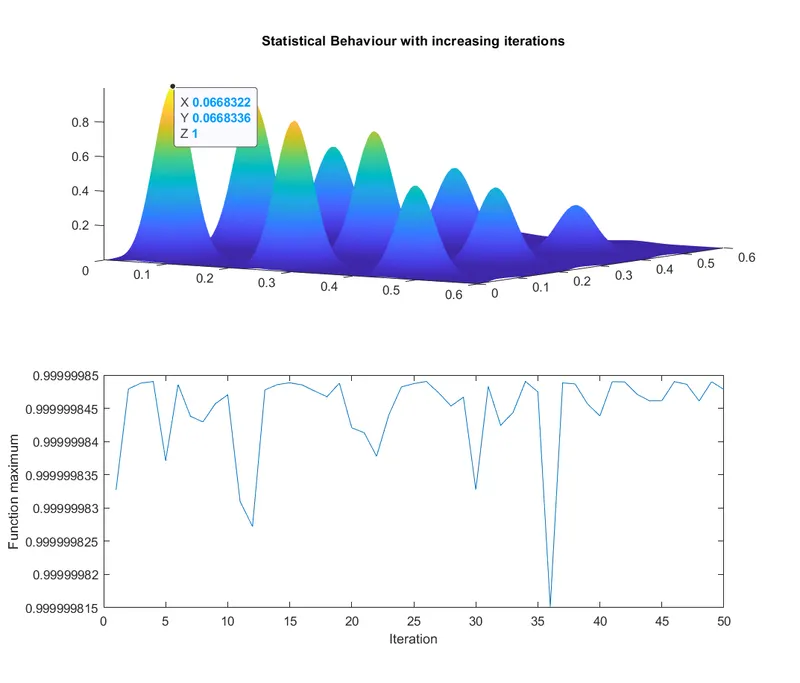
figure. Statistical Behaviour with increasing iterations
In the third study the global maximum obtained is accurate and is narrowed down ta a value of 0.999999 as shown in tha graph.
This third study time is 20.1442 seconds.
ERROR:-
While programming faced error in program second study i accidentally write input instead of inputs.
MATLAB is very good software this software alert me,
Error using input
The first argument to INPUT must be a string or character vector.
Error in statistics (line 29)
xopt(i)=input(1);
Then i corrected my mistake and i used 'inputs' word.