Week 5 - Curve fitting
CURVE FITTING USING PHYTHON
1.AIM
To understand more about linear and cubic curve fitting
2.OBJECTIVE
To compare linear and cubic curve fit and to find the best fit
To find a perfect curve fit
3.GOVERNING EQUATIONS
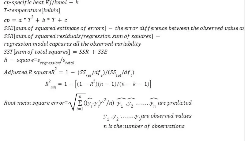
4.DESCRIPTION
Curve Fitting is the process of constructing a curve or mathematical function that best fits a series of data points,possibly subjected to constraints.
The curve fit command lets you perform exploratory data analysis, preprocess and post-process data, and compare candidate models.
It can be used to conduct regression analysis using the library of linear and nonlinear models provided or specify your own custom equations. The library provides optimized solver parameters and starting conditions to improve the quality of your fit.
Goodness of fit
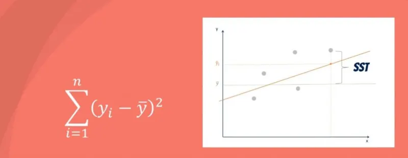
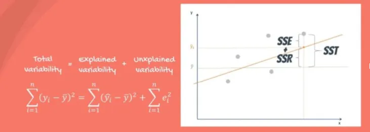
SST
The sum of squares total, denoted SST, is the squared differences between the observed dependent variable and its means
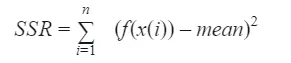
SSR
sum of squares due to regression, or SSR. It is the sum of the differences between the predicted value and the mean of the dependent variable.

If this value of SSR is equal to the sum of squares total, it means our regression model captures all the observed variability and is perfect.
SSE [ sum of squares error]
The error is the difference between the observed value and the predicted value.

To minimise the error. The smaller the error, the better the estimation power of the regression. It is also known as RSS or residual sum of squares. Residual as in remaining or unexplained.
SST = SSR + SSE.
R-Squared (R² or the coefficient of determination)
R-squared shows how well the data fit the regression model (the goodness of fit).The most common interpretation of r-squared is how well the regression model fits the observed data. Generally, a higher r-squared indicates a better fit for the model.Sometimes, a high r-squared can indicate the problems with the regression model.
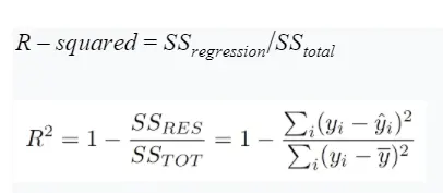
SSregression is the sum of squares due to regression (explained sum of squares)
SStotal is the total sum of squares[SST].
The sum of squares due to regression measures how well the regression model represents the data that were used for modeling. The total sum of squares measures the variation in the observed data (data used in regression modeling).
Adjusted R-Square
R2 shows how well terms (data points) fit a curve or line. Adjusted R2 also indicates how well terms fit a curve or line, but adjusts for the number of terms in a model. If you add more and more useless variables to a model, adjusted r-squared will decrease. ... n is the number of points in your data sample.

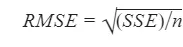
RMSE
It is the square root of the variance of the residuals. It indicates the absolute fit of the model to the data–how close the observed data points are to the model's predicted values. Whereas R-squared is a relative measure of fit, RMSE is an absolute measure of fit.
QUESTION 1;WHAT DOES PCOV AND POPT MEAN
ANS:
popt- An array of optimal values for the parameters which minimizes the sum of squares of residuals.
pcov-2d array which contains the estimated covariance of popt. The diagonals provide the variance of the parameter estimate.
EXAMPLE
def line(x, a, b):
return a * x + b
The arguments to the function should be x, followed by the parameters. We can now call curve_fit to find the best-fit parameters using a least-squares fit:
popt, pcov = curve_fit(line, x, y)
The curve_fit function returns two items, which we can popt and pcov. The popt argument are the best-fit parameters for a and b:
popt
array([ 2.99069214, 2.45335655])
which is close to the initial values of 3 and 2 used in the definition of y.
The reason the values are not exact is because there are only a limited number of random samples, so the best-fit slope is not going to be exactly those used in the definition of y. The pcov variable contains the covariance matrix, which indicates the uncertainties and correlations between parameters. This is mostly useful when the data has uncertainties
QUESTION2;WHAT DOES NP.(TEMPERATURE) DO?
NumPy is a Python library used for working with arrays.It also has functions for working in the domain of linear algebra, fourier transform, and matrices.NumPy stands for Numerical Python.
np.array(temperature) is used for accessing individual elements of temperature array in data
Numpy is imported in python as np
QUESTION3; WHAT DOES *IN *POPT MEANS ?
The star i.e * in "popt' unpacks the 'popt' array so that the optimized coefficients (parameters) values can be accessed from the array 'popt. In other words, '* (* means all) aids in referring to all the values stored in the array 'popt.
QUESTION4: CODE TO FIT A LINEAR AND CUBIC POLYNOMIAL FOR THE CP DATA .EXPLAIN DATA IS GOOD OR BAD
#program to perform curve fitting using linear and cubic curve fit

import math
import matplotlib.pyplot as plt
import numpy as np
from scipy.optimize import curve_fit

#reading the temperature cp data
def read_file():
	temperature=[]
	cp=[]

	#for read the datas line by line
	for line in open('data','r'):
		values=line.split(',')
		temperature.append(float(values[0]))
		cp.append(float(values[1]))
	return[temperature,cp]

#calling the funtion
temperature,cp=read_file()

#curve fitting using Linearpolynomial
#Function to define the linear polynomial for curve fit
def linear(T,a,b):
	return(a*T+b)
#linear=a*T+b

popt1,pcov1=curve_fit(linear,temperature,cp)
linear_fit_cp=linear(np.array(temperature),*popt1)

#maximum percentage error
error1=(np.array(np.array(cp)-np.array(linear_fit_cp)))*100/(np.array(cp))
max_error1=max(error1)

print('max %  error for curvefit using linear polynomial=',max_error1)
print('\n')

#comparing original data with curve fit usinglinear polynomial
plt.figure(1)
plt.plot(temperature,cp,color='r',linewidth=2,label='original data')
plt.plot(temperature,linear_fit_cp,color='b',linewidth=2,label='curve_fit')
plt.title('comparison of original data set and curve fit using linear_fit_cp')
plt.xlabel('temperature[k]')
plt.ylabel('specific_heat[kj/kg-k]')
plt.legend(loc='lower right')
plt.show()

#Function to define the cubic polynomial for curve fit
def cubic(T,a,b,c,d):
	return(a*pow(T,3)+b*pow(T,2)+c*T+d)
#linear=a*T+b

popt2,pcov2=curve_fit(cubic,temperature,cp)
cubic_fit_cp=cubic(np.array(temperature),*popt2)

#maximum percentage error
error2=(np.array(np.array(cp)-np.array(cubic_fit_cp)))*100/(np.array(cp))
max_error2=max(error2)

print('max %  error for curvefit using cubic polynomial=',max_error2)
print('\n')

#comparing original data with curve fit usinglinear polynomial
plt.figure(2)
plt.plot(temperature,cp,color='r',linewidth=2,label='original data')
plt.plot(temperature,cubic_fit_cp,color='b',linewidth=2,label='curve_fit')
plt.title('comparison of original data set and curve fit using cubic_fit_cp')
plt.xlabel('temperature[k]')
plt.ylabel('specific_heat[kj/kg-k]')
plt.legend(loc='lower right')
plt.show()
ALGORITHM
Step1;start sublime text
Step2;import math. command is used to call trigonometric functions(mathematical function) and step3:import matplotlib.pyplot as plt command to plot graphs in programing
Step4;numpy is a python library used for working with arrays.mathematical and logical operations on array can be performed
Step5;import scipy is used to perform curve fitting operation by importing it as an optimization function.
Step6;defined function called read_ file()to read named ‘DATA’.
Step7:where temperature and cp are extracted and values are splitted using command split defining boundary ‘,’
Step8;function read_file() is called to get array of temperature and cp .using command append each values are extracted from the file and added and returned values
Step9;defined a function which is linear polynomial where a and b are constant
Step10;popt is the command used to best value coefficients of a and b values pcov is estimated value of covariance of coefficients .
Step11;curve_fit is the inbuilt function used to find pcov and popt and .The new value of cp according to the linear polynomial ie,linear fit cp is calculated by calling the function linear and passing temperature array elements wise using numpy module and all coefficient of the linear polynomial using *popt as an input argument.
Step12;error is found out using max error percentage equation between cp and linear cp
Step13;compare the curve using plot commands
Cubic polynomial
Step11;curve_fit is the inbuilt function used to find pcov and popt and .The new value of cp according to the cubic polynomial ie,linear fit cp is calculated by calling the function cubic and passing temperature array elements wise using numpy module and all coefficient of the cubic polynomial using *popt as an input argument.
Step12;error is found out using max error percentage equation between cp and cubic cp
Step13;compare the curve using plot commands
OUTPUT
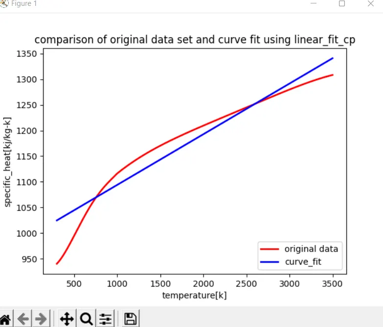
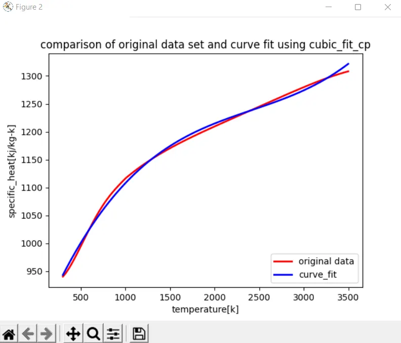

COMPARISON OF LINEAR AND CUBIC FIT
#program to perform curve fitting using linear and cubic curve fit

import math
import matplotlib.pyplot as plt
import numpy as np
from scipy.optimize import curve_fit

#reading the temperature cp data
def read_file():
	temperature=[]
	cp=[]

	#for read the datas line by line
	for line in open('data','r'):
		values=line.split(',')
		temperature.append(float(values[0]))
		cp.append(float(values[1]))
	return[temperature,cp]

#calling the funtion
temperature,cp=read_file()

#curve fitting using Linearpolynomial
#Function to define the linear polynomial for curve fit
def linear(T,a,b):
	return(a*T+b)
#cp= a*T+b

popt1,pcov1=curve_fit(linear,temperature,cp)
linear_fit_cp=linear(np.array(temperature),*popt1)

n=len(temperature)
#number of independent variable
k=0
#godness of curve fit
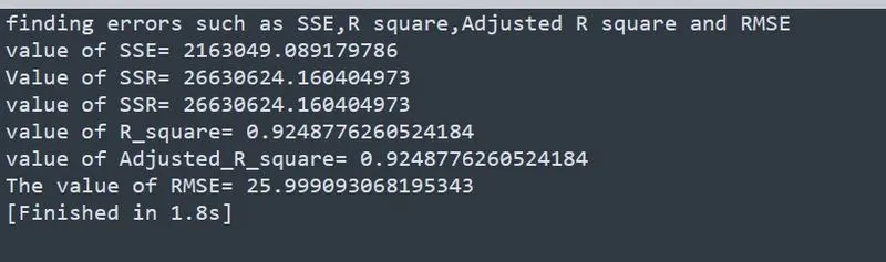
print('finding errors such as SSE,R square,Adjusted R square and RMSE')
#SSE
SSE=np.sum(pow(np.array((np.array(cp)-np.array(linear_fit_cp))),2))
print('value of SSE=',SSE)
#SSR
SSR=np.sum(pow(np.array((np.array(linear_fit_cp)-np.mean(cp))),2))
print('Value of SSR=',SSR)
#SST
SST=SSE+SSR
print('value of SSR=',SSR)
#R SQUARE
R_square=SSR/SST
print('value of R_square=',R_square)
#Adjusted R Square
Adjusted_R_square=1-((1-R_square)*(n-1)/(n-k-1))
print('value of Adjusted_R_square=',Adjusted_R_square)
#RMSE
RMSE=np.sqrt((np.sum(pow((np.array(np.array(cp)-np.array(linear_fit_cp))),2)))/n);
print('The value of RMSE=',RMSE)
import math
import matplotlib.pyplot as plt
import numpy as np
from scipy.optimize import curve_fit

#reading the temperature cp data
def read_file():
	temperature=[]
	cp=[]

	#for read the datas line by line
	for line in open('data','r'):
		values=line.split(',')
		temperature.append(float(values[0]))
		cp.append(float(values[1]))
	return[temperature,cp]

#calling the funtion
temperature,cp=read_file()

n=len(temperature)
#number of independent variable
k=0

def cubic(T,a,b,c,d):
	return(a*pow(T,3)+b*pow(T,2)+c*T+d)
#linear=a*T+b

popt2,pcov2=curve_fit(cubic,temperature,cp)
cubic_fit_cp=cubic(np.array(temperature),*popt2)

n=len(temperature)
#number of independent variable
k=0
#godness of curve fit
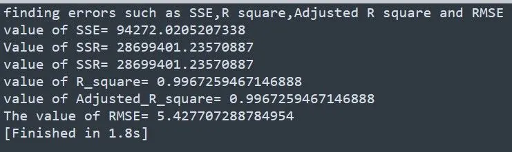
print('finding errors such as SSE,R square,Adjusted R square and RMSE')
#SSE
SSE=np.sum(pow(np.array((np.array(cp)-np.array(cubic_fit_cp))),2))
print('value of SSE=',SSE)
#SSR
SSR=np.sum(pow(np.array((np.array(cubic_fit_cp)-np.mean(cp))),2))
print('Value of SSR=',SSR)
#SST
SST=SSE+SSR
print('value of SSR=',SSR)
#R SQUARE
R_square=SSR/SST
print('value of R_square=',R_square)
#Adjusted R Square
Adjusted_R_square=1-((1-R_square)*(n-1)/(n-k-1))
print('value of Adjusted_R_square=',Adjusted_R_square)
#RMSE
RMSE=np.sqrt((np.sum(pow((np.array(np.array(cp)-np.array(cubic_fit_cp))),2)))/n);
print('The value of RMSE=',RMSE)
ALGORITHAM
Step1;start sublime text
Step2;import math. command is used to call trigonometric functions(mathematical function) and step3:import matplotlib.pyplot as plt command to plot graphs in programing
Step4;numpy is a python library used for working with arrays.mathematical and logical operations on array can be performed
Step5;import scipy is used to perform curve fitting operation by importing it as an optimization function.
Step6;defined function called read_ file()to read named ‘DATA’.
Step7:where temperature and cp are extracted and values are splitted using command split defining boundary ‘,’
Step8;function read_file() is called to get array of temperature and cp .using command append each values are extracted from the file and added and returned values
Step9;defined a function which is linear polynomial where a and b are constant
Step10;popt is the command used to best value coefficients of a and b values pcov is estimated value of covariance of coefficients .
Step11;curve_fit is the inbuilt function used to find pcov and popt and .The new value of cp according to the linear polynomial ie,linear fit cp is calculated by calling the function linear and passing temperature array elements wise using numpy module and all coefficient of the linear polynomial using *popt as an input argument.
Step12;find errors like SSE SSR R Square Adjusted R square using respective equations and compare the output of linear and cubic data
OUTPUT
QUESTION NUMBER5 : HOW TO MAKE CURVE FIT PERFECCT
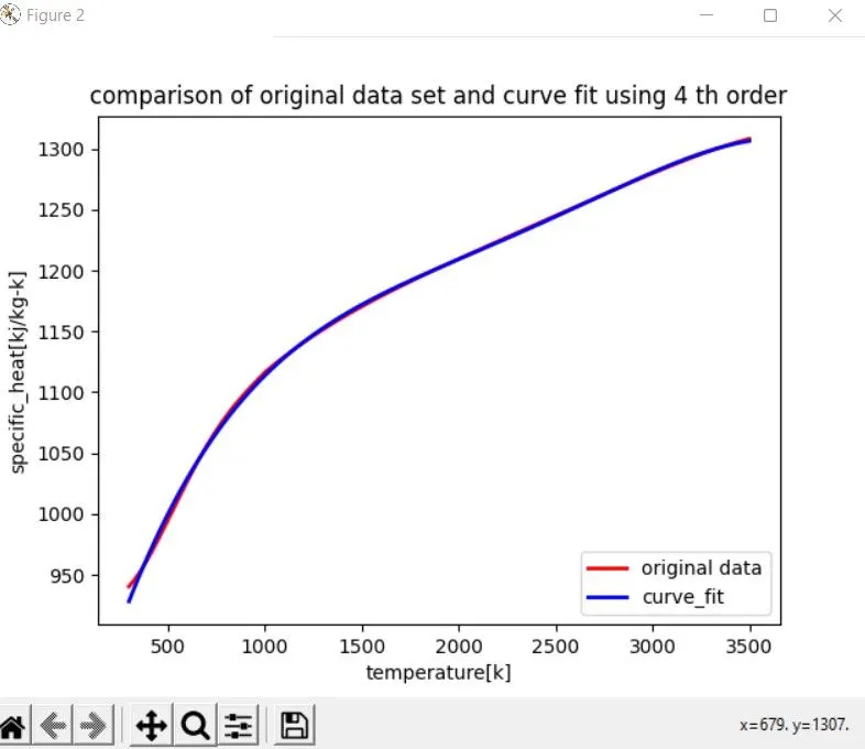
INCREASE THE ODER OF THE POLYNOMIAL
As the order increases the fit of curve also increases
USE SPLIT WISE METHOD
As the number of splits increases fit of curve increases
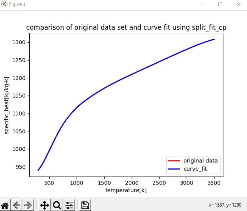
split wise method is more effective than normal cubic /linear fit curve
QUESTION NUMBER6:SHOW EMPIRICALLY AS TO HOW WELL YOUR CURVE HAS BEEN FIT
#splitwisemethod
import math
import matplotlib.pyplot as plt
import numpy as np
from scipy.optimize import curve_fit

#reading the temperature cp data
def read_file():
	temperature=[]
	cp=[]

	#for read the datas line by line
	for line in open('data','r'):
		values=line.split(',')
		temperature.append(float(values[0]))
		cp.append(float(values[1]))
	return[temperature,cp]

#calling the funtion
temperature,cp=read_file()


temperature1=temperature[0:200]
cp1=cp[0:200]
temperature2=temperature[200:400]
cp2=cp[200:400]
temperature3=temperature[400:600]
cp3=cp[400:600]
temperature4=temperature[600:800]
cp4=cp[600:800]
temperature5=temperature[800:1000]
cp5=cp[800:1000]
temperature6=temperature[1000:1200]
cp6=cp[1000:1200]
temperature7=temperature[1200:1400]
cp7=cp[1200:1400]
temperature8=temperature[1400:1600]
cp8=cp[1400:1600]
temperature9=temperature[1600:1800]
cp9=cp[1600:1800]
temperature10=temperature[1800:2000]
cp10=cp[1800:2000]
temperature11=temperature[2000:2200]
cp11=cp[2000:2200]
temperature12=temperature[2200:2400]
cp12=cp[2200:2400]
temperature13=temperature[2400:2600]
cp13=cp[2400:2600]
temperature14=temperature[2600:2800]
cp14=cp[2600:2800]
temperature15=temperature[2800:3000]
cp15=cp[2800:3000]
temperature16 =temperature[3000:3200]
cp16=cp[3000:3200]

#curvefitting use split wise
def cubic(T,a,b,c,d):
	return(a*pow(T,3)+b*pow(T,2)+c*T+ d)


popt1,pcov1=curve_fit(cubic,temperature1,cp1)
cubic_fit_cp1=cubic(np.array(temperature1),*popt1)

popt2,pcov2=curve_fit(cubic,temperature2,cp2)
cubic_fit_cp2=cubic(np.array(temperature2),*popt2)

popt3,pcov3=curve_fit(cubic,temperature3,cp3)
cubic_fit_cp3=cubic(np.array(temperature3),*popt3)

popt4,pcov4=curve_fit(cubic,temperature4,cp4)
cubic_fit_cp4=cubic(np.array(temperature4),*popt4)

popt5,pcov5=curve_fit(cubic,temperature5,cp5)
cubic_fit_cp5=cubic(np.array(temperature5),*popt5)

popt6,pcov6=curve_fit(cubic,temperature6,cp6)
cubic_fit_cp6=cubic(np.array(temperature6),*popt6)

popt7,pcov7=curve_fit(cubic,temperature7,cp7)
cubic_fit_cp7=cubic(np.array(temperature7),*popt7)

popt8,pcov8=curve_fit(cubic,temperature8,cp8)
cubic_fit_cp8=cubic(np.array(temperature8),*popt8)

popt9,pcov9=curve_fit(cubic,temperature9,cp9)
cubic_fit_cp9=cubic(np.array(temperature9),*popt9)

popt10,pcov10=curve_fit(cubic,temperature10,cp10)
cubic_fit_cp10=cubic(np.array(temperature10),*popt10)


popt11,pcov11=curve_fit(cubic,temperature11,cp11)
cubic_fit_cp11=cubic(np.array(temperature11),*popt11)

popt12,pcov12=curve_fit(cubic,temperature12,cp12)
cubic_fit_cp12=cubic(np.array(temperature12),*popt12)

popt13,pcov13=curve_fit(cubic,temperature13,cp13)
cubic_fit_cp13=cubic(np.array(temperature13),*popt13)

popt14,pcov14=curve_fit(cubic,temperature14,cp14)
cubic_fit_cp14=cubic(np.array(temperature14),*popt14)

popt15,pcov15=curve_fit(cubic,temperature15,cp15)
cubic_fit_cp15=cubic(np.array(temperature15),*popt15)

popt16,pcov16=curve_fit(cubic,temperature16,cp16)
cubic_fit_cp16=cubic(np.array(temperature16),*popt16)

#string concatenate is joining character string
split_fit_cp=np.concatenate((cubic_fit_cp1,cubic_fit_cp2,cubic_fit_cp3,cubic_fit_cp4,cubic_fit_cp5,cubic_fit_cp6,cubic_fit_cp7,cubic_fit_cp8,cubic_fit_cp9,cubic_fit_cp10,cubic_fit_cp11,cubic_fit_cp12,cubic_fit_cp13,cubic_fit_cp14,cubic_fit_cp15,cubic_fit_cp16))


#comparing original data with curve fit usinglinear polynomial
plt.figure()
plt.plot(temperature,cp,color='r',linewidth=2,label='original data')
plt.plot(temperature,split_fit_cp,color='b',linewidth=2,label='curve_fit')
plt.title('comparison of original data set and curve fit using split_fit_cp')
plt.xlabel('temperature[k]')
plt.ylabel('specific_heat[kj/kg-k]')
plt.legend(loc='lower right')
plt.show()
OUTPUT
OUT PUT OF HIGHER ORDER CURVE FIT
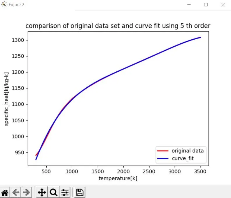
conclusion from these observations
Fifth Order is more fit than fourth order curve fit