Week 4.1 - Genetic Algorithm

GENETIC ALGORITHAM

AIM

A code in Matlab to optimise the given stalagmite function and find the global maxima of the function

DESCRIPTION

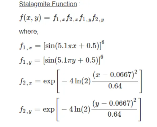
STALAGMITE FUNCTION

1.Stalagmite are structures formed from mineral deposits that hang from caves. These formations hold tightly to the ceiling and hang down. Stalagmite and Stalactite functions are mathematical functions which represents shapes similar to that of the stalagmite and stalactite functions

2.A Stalagmite function refers to the function which are generally values over a stalagmite kind of surface of finding out the local and global maxima and minima of a particular given function.

OPTIMISATION

It is done by symmetrically choosing input values from within an allowed set and computing the result of the function.

Set optimization options to use the interior-point algorithm and display the results at each iteration.

Optimization refers to finding the values of inputs in such a way that we get the "best" output values. The definition of "best" varies from problem to problem, but in mathematical terms, it refers to maximizing or minimizing one or more objective functions, by varying the input parameters.

The set of all possible solutions or values which the inputs can take make up the search space. In this search space, lies a point or a set of points which gives the optimal solution. The aim of optimization is to find that point or set of points in the search space.

Example;

Set options for ga by using optimoptions.

options = optimoptions('ga','Option1','value1','Option2','value2');

Options=optimoptions('fmincon','Algorithm','interior-point','Display','iter');

optimization provides functions for finding parameters that minimize or maximize objectives while satisfying constraints. The toolbox includes solvers for linear programming (LP), mixed-integer linear programming (MILP), quadratic programming (QP), second-order cone programming (SOCP), nonlinear programming (NLP), constrained linear least squares, nonlinear least squares, and nonlinear equations.

You can define your optimization problem with functions and matrices or by specifying variable expressions that reflect the underlying mathematics. You can use automatic differentiation of objective and constraint functions for faster and more accurate solutions.

options = optimoptions(@ga,'UseVectorized',true);

PlotFcn specifies the plot function or functions called at each iteration by ga or gamultiobj. Set the PlotFcn option to be a built-in plot function name or a handle to the plot function. You can stop the algorithm at any time by clicking the Stop button on the plot window. For example, to display the best function value, set options as follows:

options = optimoptions('ga','PlotFcn','gaplotbestf');

To display multiple plots, use a cell array of built-in plot function names or a cell array of function handles:

options = optimoptions('patternsearch','PlotFcn', {@plotfun1, @plotfun2, ...});

where @plotfun1, @plotfun2, and so on are function handles to the plot functions. If you specify more than one plot function, all plots appear as subplots in the same window. Right-click any subplot to obtain a larger version in a separate figure window.

Ensure that you pass options to the solver. Otherwise, patternsearch uses the default option values.

GENETIC ALGORITHM

A genetic algorithm (GA) is a method for solving both constrained and unconstrained optimization problems based on a natural selection process that mimics biological evolution. The algorithm repeatedly modifies a population of individual solutions. At each step, the genetic algorithm randomly selects individuals from the current population and uses them as parents to produce the children for the next generation. Over successive generations, the population "evolves" toward an optimal solution

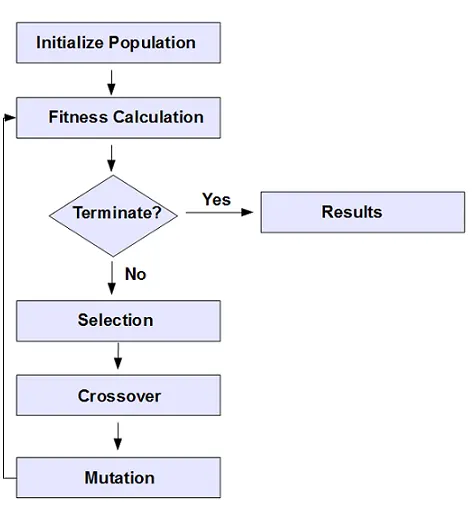
The following outline summarizes how the genetic algorithm works:

1.The algorithm begins by creating a random initial population.

2. The algorithm then creates a sequence of new populations.

At each step ,the algorithm uses the individual in the current generation to create the next Population.to create the new population ,the algorithm performs the following

1.Scores each member of the current population by computing its fitness value. These values are called the raw fitness scores.

2.Scales the raw fitness scores to convert them into a more usable range of values. These scaled values are called expectation values.

3.Selects members, called parents, based on their expectation.

4.Some of the individuals in the current population that have lower fitness are chosen as elite. These elite individuals are passed to the next population.

5.Produces children from the parents. Children are produced either by making random changes to a single parent— mutation—or by combining the vector entries of a pair of parents—crossover.

6.Replaces the current population with the children to form the next generation.

7.The algorithm stops when criteria is met

Stopping Conditions for the Algorithm

The genetic algorithm uses the following options to determine when to stop. See the default values for each option by running opts = optimoptions('ga').

• MaxGenerations — The algorithm stops when the number of generations reaches MaxGenerations.
• MaxTime — The algorithm stops after running for an amount of time in seconds equal to MaxTime.
• FitnessLimit — The algorithm stops when the value of the fitness function for the best point in the current population is less than or equal to FitnessLimit.
• MaxStallGenerations — The algorithm stops when the average relative change in the fitness function value over MaxStallGenerations is less than Function tolerance.
• MaxStallTime — The algorithm stops if there is no improvement in the objective function during an interval of time in seconds equal to MaxStallTime.
• FunctionTolerance — The algorithm runs until the average relative change in the fitness function value over MaxStallGenerations is less than Function tolerance.
• ConstraintTolerance — The ConstraintTolerance is not used as a stopping criterion. It is used to determine the feasibility with respect to nonlinear constraints. Also, max(sqrt(eps),ConstraintTolerance) determines feasibility with respect to linear constraints.

The algorithm stops as soon as any one of these conditions is met.

Creating the Next Generation

At each step, the genetic algorithm uses the current population to create the children that make up the next generation. The algorithm selects a group of individuals in the current population, called parents, who contribute their genes—the entries of their vectors—to their children. The algorithm usually selects individuals that have better fitness values as parents. You can specify the function that the algorithm uses to select the parents in the SelectionFcn option. See Selection Options.

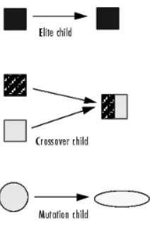
The genetic algorithm creates three types of children for the next generation:

• Elite are the individuals in the current generation with the best fitness values. These individuals automatically survive to the next generation.
• Crossovers are created by combining the vectors of a pair of parents.
• Mutation children are created by introducing random changes, or mutations, to a single parent.

The following schematic diagram illustrates the three types of children.

[x,fval] = ga(fun,x0,A,b,Aeq,beq,lb,ub,nonlcon,options)

[x,fval] = ga(FitnessFunction,numberOfVariables,[],[],[],[],lb,ub)

The format for writing genetic algorithm in MATLAB is as follows:

x = ga(fun,nvars, A, b, Aeq, beq, lb, ub,nonlcon, options)

1. x is the local minimum point.
2. fun is the function to be called. (In our case, it's the stalagmite function)
3. nvars indicates the number of variables used.
4. A and b are used to indicate any kind of inequalities that exist in the function.
5. Aeq and Beq also denote the inequalities.
6. lb= lower bound.
7. ub= upper bound.
8. nonlcon gives two vectors representing inequalities and equalities.
9. options are used to perform additional operations like increasing population size. This is done with the help of "optimoptions".OBJECTIVES OF THE PROJECT

   Write a code in MATLAB to optimise the stalagmite function and find the global maxima of the function

   • Clearly explain the concept of genetic algorithm in your own words and also explain the syntax for ga in Matlab.
   • Plot graphs for all 3 studies and for maximum no.of iterations

ALGORITHM

Step1;use commands to clear and close all windows

Step2;x is assigned to 150( size of array) values using linspace command

Step3; y is assigned to 150 values using linspace command

Step4;numcases set to 50 that ga will run upto 50 cases(ga algorithm function does not have an idea to when to stop and start)

Step5;initiated a stalagmite function called using get_stalagmite command to generate it.

For study1

Step6;to find statistical behaviour

Step7;for loop initialized to num_cases

Step8; genetic algorithm of stalagmite function with variable 2 initialized using command ga(@stalagmite,2)

Step9;the gas syntax used first study unbounded inputs x=ga(fun,nvars),Genetic algorithm is an inbuilt function in matlab,nvars is no.of variables=2(x and y)

Step9;fopt is optimum values of function creates

Step10;x optimum values find out using xopt(i) from inputs(1)

Step12;figure 1 command initialized

Step11;subplot commands used to plot two different plots in single frame

Step13;surf c a plot of 3d using x y f plotted

step14;Shading interp used to remove grid and smooth plot

step15;Plot3 command used to plot 3D of x optimum y optimum and z optimum

step16;Title of unbounded inputs given by command title

Step17;subplot initiated to plot second graph of f optimum

step18;Plot of f optimum

Step19;input X label and y label

Step20;study times commands tic and toc commands are used

STUDY2

Step21;genetic algorithm initiated asx=ga(fun,nvars,A,b,Aeq,beq,lb,ub) as upper and lower bounds

ga(@stalagmite_fun,2.[],[],[],[],[0;0],[1;1])

[][] no linear inequalities exist between x and y

[][] are used because no linear inequalities exist between x equation and y equation

[0;0] define lower boundary between x and y

[1;1]defines the upper boundary condition between x and y

Step22;optimoptions are used to change the syntax of ga

step23;Population size increased to 170

Step24;to measure how much time is taken to complete the study tic and toc command has been used

STUDY3

Step24;to increase size of population using population size

step25;x=ga(fun,nvars,A,b,Aeq,Beq,lb,ub,nonclon,intcon,options)

PROBLEM

PROGRAM

clear all

close all

clc

%defining our search space

x=linspace(0,0.6,150);

y=linspace(0,0.6,150);

%assigning 50 cases

num_cases=50

%stalagmite function initialization

[xx yy]=meshgrid(x,y);

for i=1:length(xx)

for j=1:length(yy)

input_vector(1)=xx(i,j);

input_vector(2)=yy(i,j);

f(i,j)=stalagmite(input_vector);

end

end

surfc(xx,yy,f)

shading interp

[input,fopt]=ga(@stalagmite,2)

%study1 _bound

tic

for i=1:num_cases

[input,fopt(i)]=ga(@stalagmite,2)

xopt(i)=input(1);

yopt(i)=input(2);

end

study1_time1=toc

%figure(1) from study1

figure(1)

subplot(2,1,1)

surfc(x,y,-f)

shading interp

hold on

plot3(xopt,yopt,-fopt,'marker','o')

subplot(2,1,2)

plot(-fopt)

title('unbounded inputs')

xlabel('iteration')

ylabel('function maximum')

tic

%study2-bounded (with upper and lower bound)

for i=1:num_cases

[input,fopt(i)]=ga(@stalagmite,2,[],[],[],[],[0;0],[0.6;0.6]);

xopt(i)=input(1);

yopt(i)=input(2);

end

study_time2=toc

figure(2)

subplot(2,1,1)

surfc(x,y,-f)

shading interp

hold on

plot3(xopt,yopt,-fopt,'marker','o')

subplot(2,1,2)

plot(-fopt)

xlabel('iteration')

ylabel('function maximum')

%study3-increased initial population

tic

options=optimoptions('ga')

options=optimoptions(options,'populationsize',250)

for i=1:num_cases

[input,

fopt(i)]=ga(@stalagmite,2,[],[],[],[],[0;0],[0.6;0.6],[],[],options)

xopt(i)=input(1)

yopt(i)=input(2)

end

study_time3=toc

figure(3)

subplot(2,1,1)

surf(x,y,-f)

shading interp

hold on

plot3(xopt,yopt,-fopt,'marker','o')

subplot(2,1,2)

plot(-fopt)

xlabel('iteration')

ylabel('function maximum')

INITIALISING STALAGMITE FUNCTION

clear all

close all

clc

%defining our search space

x=linspace(0,0.6,150);

y=linspace(0,0.6,150);

[xx yy]=meshgrid(x,y);

%creating the stalagmite function

for i=1:length(xx)

for j=1:length(yy)

input_vector(1)=xx(i,j);

input_vector(2)=yy(i,j);

f(i,j)=stalagmite(input_vector);

end

end

surfc(xx,yy,f)

shading interp

[input,fopt]=ga(@stalagmite,2)

OUTPUT

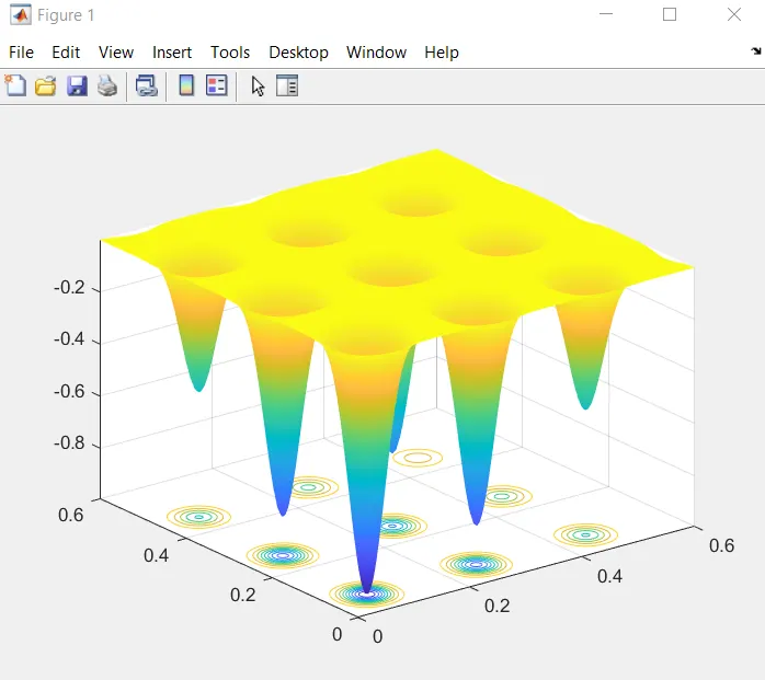
STALAGMITE FUNCTION

unction [f]=stalagmite(input_vector)

x=input_vector(1)

y=input_vector(2)

f1x= (sin(5.1*pi*x+0.5)).^6;

f1y= (sin(5.1*pi*y+0.5)).^6;

f2x=exp(-4*log(2)*(x-0.0667).^2/0.64)

f2y=exp(-4*log(2)*(y-0.0667).^2/0.64)

f= -1*(f1x*f2x*f1y*f2y);

end

OUTPUTS

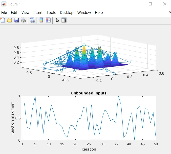
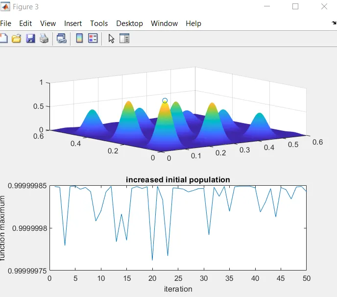
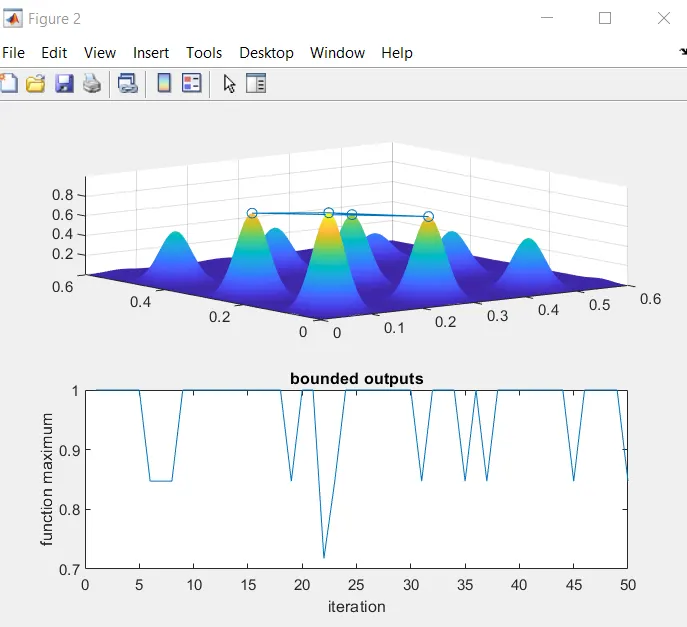
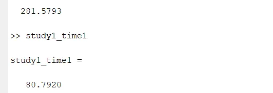
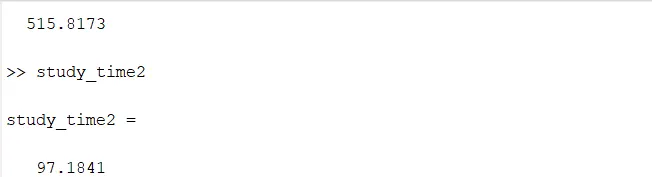
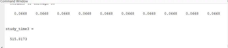
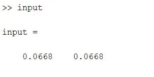
VALUE OF X OR Y MAXIMUM

clear all
close all
clc

%defining our search space
x=linspace(0,0.6,150);
y=linspace(0,0.6,150);
%assigning 50 cases
num_cases=50
%stalagmite function initilization
[xx yy]=meshgrid(x,y);
for i=1:length(xx)
    for j=1:length(yy)
        input_vector(1)=xx(i,j);
        input_vector(2)=yy(i,j);
        f(i,j)=stalagmite(input_vector);
    end
end

surfc(xx,yy,f)
shading interp
[input,fopt]=ga(@stalagmite,2)


%study1 _bound
tic
for i=1:num_cases
    [input,fopt(i)]=ga(@stalagmite,2)
    xopt(i)=input(1);
    yopt(i)=input(2);
end
study1_time1=toc
%figure(1) from study1
figure(1)
subplot(2,1,1)
surfc(x,y,-f)
shading interp
hold on
plot3(xopt,yopt,-fopt,'marker','o')
subplot(2,1,2)
plot(-fopt)
title('unbounded inputs') 
xlabel('iteration')
ylabel('function maximum')
tic

%study2-bounded (with upper and lower bound)
%initiated loop

for i=1:num_cases
    [input,fopt(i)]=ga(@stalagmite,2,[],[],[],[],[0;0],[0.6;0.6]);
    xopt(i)= input(1);
    yopt(i)= input(2);
end
study_time2 = toc
figure(2)
subplot(2,1,1)
surfc(x,y,-f)

shading interp
hold on
plot3(xopt,yopt,-fopt,'marker','o')
subplot(2,1,2)
plot(-fopt)
title('bounded outputs')
xlabel('iteration')
ylabel('function maximum')
%study3-increased initial population
tic
options=optimoptions('ga')
options=optimoptions(options,'populationsize',250)
for i=1:num_cases
    [input,fopt(i)]=ga(@stalagmite,2,[],[],[],[],[0;0],[0.6;0.6],[],[],options)
    xopt(i)= input(1)
    yopt(i)= input(2)
end
study_time3 =toc
figure(3)
subplot(2,1,1)
surf(x,y,-f)

shading interp
hold on
plot3(xopt,yopt,-fopt,'marker','o')
subplot(2,1,2)
plot(-fopt)
title('increased initial population')
xlabel('iteration')
ylabel('function maximum')

SUBPLOT1
%stalagmite function

function [f]=stalagmite(input_vector)
       x=input_vector(1)
       y=input_vector(2)
     f1x= (sin(5.1*pi*x+0.5)).^6;
     f1y= (sin(5.1*pi*y+0.5)).^6;
     f2x=exp(-4*log(2)*(x-0.0667).^2/0.64)
     f2y=exp(-4*log(2)*(y-0.0667).^2/0.64)
     f= -1*(f1x*f2x*f1y*f2y);
   
end
SUBPLOT2

clear all
close all
clc

%defining our search space
x=linspace(0,0.6,150);
y=linspace(0,0.6,150);


[xx yy]=meshgrid(x,y);

%creating the salagmite function 
for i=1:length(xx)
    for j=1:length(yy)
        input_vector(1)=xx(i,j);
        input_vector(2)=yy(i,j);
        f(i,j)=stalagmite(input_vector);
    end
end
surfc(xx,yy,f)
shading interp
[input,fopt]=ga(@stalagmite,2)

CONCLUSION

Matlab program of genectic algoritham completed and executed successfully,outputs are verified