Otto cycle
OTTO CYCLE
1 AIM
To plot the pressure- volume graph of a otto cycle using Matlab
to compute Thermal efficiency of otto cycle
2 GOVERNING EQUATIONS
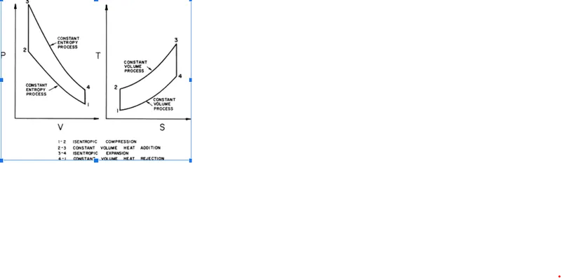
The Otto cycle is consists of
Process 1–2 is an adiabatic (isentropic) compression of the charge as the piston moves from bottom dead center (BDC) to top dead center (TDC).
Crank angle changes180 to 0
V1p1 to v2p2
Process 2–3 is a constant-volume heat transfer to the working gas from an external source while the piston is at top dead center. This process is intended to represent the ignition of the fuel-air mixture and the subsequent rapid burning.
V2p2 to v3p3
V2=V3
Process 3–4 is an adiabatic (isentropic) expansion (power stroke).
crank angle changes from 0 to 180
V3p3 tov4p4
Process 4–1 completes the cycle by a constant-volume process in which heat is rejected from the air while the piston is at the bottom dead center.
V4p4 to v1p1
V4=V1
Swept volume -volume through which a piston moves as it makes a stroke.
Clearance volume- volume between the cylinder head and the piston when the piston is at TDC
Compression ratio-The ratio of clearance volume to the swept volume determines the compression ratio of the engine.
t -is temperature in kelvin
p - pressure in pascal
v -volume
gamma -specific ratio
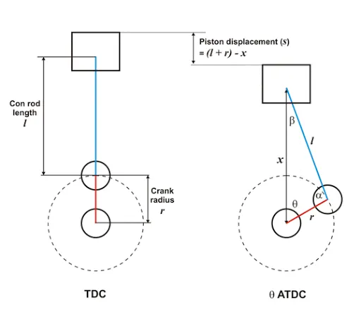
*v_swept=Pi/4*bore2*stroke
*v_clearence=v_swept/(cr-1)
*v1=v_swept+v_clearence
*v2=v_clearence
*Crank radius= crankshaft stroke/2
*Ratio(R)=connecting rod/crank radius
*p1v1=p2v2
*p1v1/t1=p2v2/t2
*Compression ratio(cr)=v1/v2
*To find volume in isentropic process
*v=(1+0.5*(cr-1)*(r+1-cosd(theta)-(r2-sind(theta)2).0.5).*v_c
*otto cycle efficiency=1-(1./(cr).^(gamma-1))
OBJECTIVES
To excecute a matlab program to find the efficency of otto cycle and to plot PV diagram using matlab
Program ALGORITHAM
Step 1;start the program
step 2 ;give common commands to clear and close all windows
step 3 ;input given state variables P1(initial pressure) ,initial temperature(t1), temperature at point 3(t3)
Enter given Engine parameters like bore,stroke ,connecting rod length and compression ratio
Step 4;calculate swept volume and clearance volume using Engine parameters
Step 5;compute state variable at each point using thermodynamic formulae
step 6;find p2 using
p1v1^gamma=p2v2^gamma ie,
p2=p1*(v1/v2)^gamma
p2 =p1*cr^gamma
Step 7;calculate t2
p1v1/t1=p2v2/t2
t2=(p2*v2*t1)/(p1*v1);
t2 =(p2*v2*t1)/(p1*v1)
step 8; calculate p3
v3=v2
p3v3/t3=p2v2/t2
p3 =p2*t3/t2
Step 9;calculate p4
v4 =v1
p4 =p3*(v3/v4)^gamma
step 10;command fig(1) inialized
step 11;hold on command is used to mark all points in a single frame
step 12;mark these points using command plot(v1,p1 ,'*','color','r')
plot(v2,p2 ,'*','color','r')
plot(v3,p3 ,'*','color','r')
plot(v4,p4 ,'*','color','r')
step 13;connecting these values using 'plot 'command [v1 v2 v3 v4][p1 p2 p3 p4] will give a straight line which is wrong
step 14;subprogram function introduced to find the which gives array of volume at each crank position to plot the graph of isentropic process to get the curve
step 15; function[v]=engine_kinematics(bore,stroke,con_rod,cr,start_crank,end_crank)
step 16;a[crank radius] & R defined
step 17;theta defined using linspace command where range comprise from start_crank to end_crannk
step 18;volume sept by curve defined by equation using v=(1+0.5*(cr-1)*(r+1-cosd(theta)-(r2-sind(theta)2).0.5).*v_c
step 19;constant defined constant_c=p1*v1^gamma,
v_compression=engine_kinematics(bore,stroke,con_rod,cr,180,0)
p_compression=constant_c./v_compression.^gamma
step 20;v expansion and p expansion defined
v_expansion=engine_kinematics(bore,stroke,con_rod,cr,0,180)
p_expansion=constant_c./v_expansion.^gamma
step 21;plot the graph using
[v1 v_compression v2 v3 v_expansion v4 v1],[p1 p_compression p2 p3 p_expansion p4 p1])
step 22;constant volume heat addition and constant volume heat rejection are connected by straight line
Step 23;plot the graph of pressure volume
Step 24;find thermal efficiency using equation 1-(1./(cr).^(gamma-1))
Step 25;end the program
PROGRAM
clear all
close all
clc
%inputs
bore=0.1
stroke=0.1
con_rod=0.1
cr=12
gamma=1.4
%state variables
p1=101325
t1=500
t3=2300
%calculate swept and clearance volume
v_swept=(pi/4)*bore^2*stroke
v_clearence=v_swept/(cr-1)
%calculate v1 and v2 using v_swept and v_clearence
v1=v_swept+v_clearence
v2=v_clearence
%calculate p2
%p1v1^gamma=p2v2^gamma
%p2=p1*(v1/v2)^gamma
p2 =p1*cr^gamma;
%calculate t2
%p1v1/t1=p2v2/t2
%t2=(p2*v2*t1)/(p1*v1);
t2 =(p2*v2*t1)/(p1*v1);
%constant_cp1v1^gamma
constant_c=p1*v1^gamma
%v_compression
% start_crank 180 to end_crank 0
v_compression=engine_kinematics(bore,stroke,con_rod,cr,180,0)
p_compression=constant_c./v_compression.^gamma
%state variable at point 3
%constant_volume process
v3 =v2;
%p3v3/t3=p2v2/t2
p3 =p2*t3/t2;
constant_c=p3*v3^gamma
v_expansion=engine_kinematics(bore,stroke,con_rod,cr,0,180)
p_expansion=constant_c./v_expansion.^gamma
%state variable at point 4
v4 =v1
p4 =p3*(v3/v4)^gamma
figure(1)
hold on
plot(v1,p1 ,'*','color','r')
plot(v_compression,p_compression)
plot(v2,p2 ,'*','color','r')
plot(v3,p3 ,'*','color','r')
plot(v_expansion,p_expansion)
plot(v4,p4 ,'*','color','r')
figure(2)
plot([v1 v_compression v2 v3 v_expansion v4 v1],[p1 p_compression p2 p3 p_expansion p4 p1])
%otto cycle efficiency
efficiency=1-(1./(cr).^(gamma-1))
SUBPROGRAM (To plot isentropic process by finding array of volume at each crank position)
function[v]=engine_kinematics(bore,stroke,con_rod,cr,start_crank,end_crank)
a=stroke/2
R=con_rod/a
v_s=pi/4*bore^2*stroke
v_c=v_s/(cr-1)
theta=linspace(start_crank,end_crank,100)
term 1=0.5*(cr-1)
term 2=R+1-cosd(theta)
term3=(R^2-sind(theta).^2).^0.5;
v=(1+term1*(term2-term3)).*v_c
End
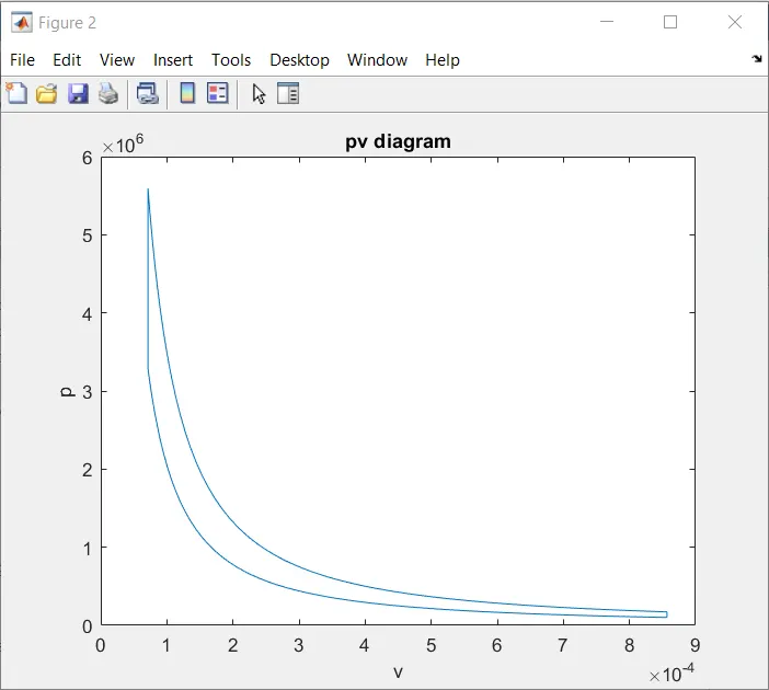
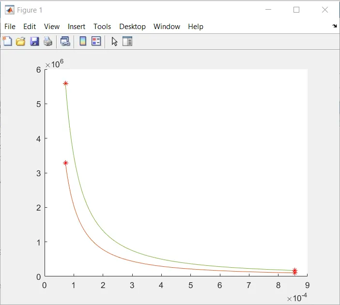
Mistake and outputs
clear all
close all
clc
%inputs
bore=0.1
stroke=0.1
con_rod=0.1
cr=12
gamma=1.4
%state variables
p1=101325
t1=500
t3=2300
%calculate swept and clearance volume
v_swept=(pi/4)*bore^2*stroke
v_clearence=v_swept/(cr-1)
%calculate v1 and v2 using v_swept and v_clearence
v1=v_swept+v_clearence
v2=v_clearence
%calculate p2
%p1v1^gamma=p2v2^gamma
%p2=p1*(v1/v2)^gamma
p2 =p1*cr^gamma;
%calculate t2
%p1v1/t1=p2v2/t2
%t2=(p2*v2*t1)/(p1*v1);
t2 =(p2*v2*t1)/(p1*v1);
%constant_cp1v1^gamma
%constant_volume process
v3 =v2;
%p3v3/t3=p2v2/t2
p3 =p2*t3/t2
%state variable at point 4
v4 =v1
p4 =p3*(v3/v4)^gamma
figure(1)
hold on
plot(v1,p1 ,'*','color','r')
plot(v2,p2 ,'*','color','r')
plot(v3,p3 ,'*','color','r')
plot(v4,p4 ,'*','color','r')
figure(2)
plot([v1 v2 v3 v4 v1],[p1 p2 p3 p4 p1])
title('pv diagram of otto cycle')
xlabel('p')
ylabel('v')
output
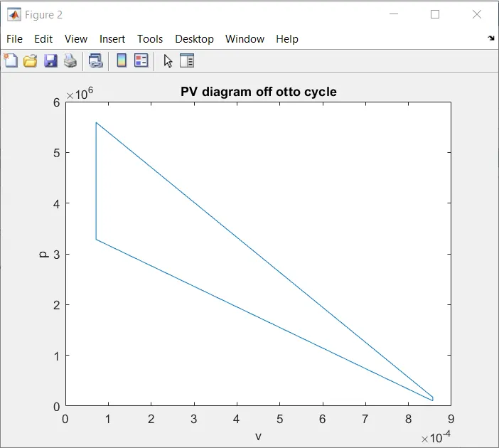
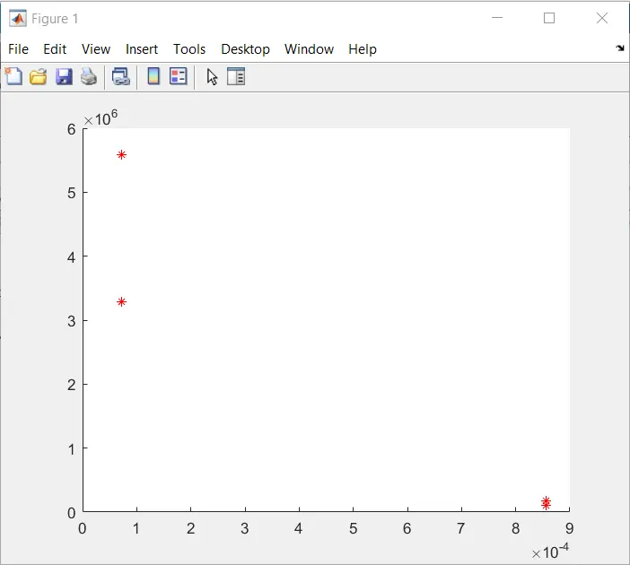
Conclusion
Pv graph of otto cycle plotted
efficency of otto cycle calulated
The matlab program has been executed successfully and output verified
Program
clear all
close all
clc
%inputs
bore=0.1
stroke=0.1
con_rod=0.1
cr=12

gamma=1.4
%state variables
p1=101325
t1=500
t3=2300

%calculate swept and clearance volume
v_swept=(pi/4)*bore^2*stroke
v_clearence=v_swept/(cr-1)

%calculate v1 and v2 using v_swept and v_clearence
v1=v_swept+v_clearence
v2=v_clearence

%calculate p2
%p1v1^gamma=p2v2^gamma
%p2=p1*(v1/v2)^gamma
p2 =p1*cr^gamma;
%calculate t2
%p1v1/t1=p2v2/t2
%t2=(p2*v2*t1)/(p1*v1);
t2 =(p2*v2*t1)/(p1*v1);

%constant_cp1v1^gamma
constant_c=p1*v1^gamma

%v_compression
%compression start_crank 180 to end_crank 0
v_compression=engine_kinematics(bore,stroke,con_rod,cr,180,0)
p_compression=constant_c./v_compression.^gamma

%state variable at point 3
%constant_volume process
v3 =v2;

%p3v3/t3=p2v2/t2
p3 =p2*t3/t2
constant_c=p3*v3^gamma
v_expansion=engine_kinematics(bore,stroke,con_rod,cr,0,180)
p_expansion=constant_c./v_expansion.^gamma
%state variable at point 4
v4 =v1
p4 =p3*(v3/v4)^gamma

figure(1)
hold on

plot(v1,p1 ,'*','color','r')
plot(v_compression,p_compression)
plot(v2,p2 ,'*','color','r')
plot(v3,p3 ,'*','color','r')
plot(v_expansion,p_expansion)
plot(v4,p4 ,'*','color','r')

figure(2)
plot([v1 v_compression v2 v3 v_expansion v4 v1],[p1 p_compression p2 p3 p_expansion p4 p1])
%otto cycle efficiency
efficiency=1-(1./(cr).^(gamma-1))

Subprogram

To plot isentropic process by finding  array of volume at each crank position

function[v]=engine_kinematics(bore,stroke,con_rod,cr,start_crank,end_crank)

 a=stroke/2
 R=con_rod/a

 v_s=pi/4*bore^2*stroke
 v_c=v_s/(cr-1)

 theta=linspace(start_crank,end_crank,100)
 term 1=0.5*(cr-1)