CURVE FITTING
CURVE FITTING
1.AIM
To plot cp -temperature data of oxygen using curve fit and to compare the linear and cubic fit curve data with original data by plotting.And to find the fitness of the curve.
3.OBJECTIVES OF THE PROJECT
A matlab program to execute curve fitting
To write a program to fit curves for linear and cubic polynomial for the cp data
To plot linear and cubic fit curves along original data
A program to find error between curve fitting and original data set[fitness of curve fitting ]
4.DESCRIPTION
Curve Fitting is the process of constructing a curve or mathematical function that best fits a series of data points,possibly subjected to constraints.
The curve fit command lets you perform exploratory data analysis, preprocess and post-process data, and compare candidate models.
It can be used to conduct regression analysis using the library of linear and nonlinear models provided or specify your own custom equations. The library provides optimized solver parameters and starting conditions to improve the quality of your fit.
Polyfit -it is a matlab function that computes a least squares polynomial for a given set of data.polyfit generates the coefficients of the polynomial which can be used to model a curve to fit the data.
polyfit() function, accepts three different input values: x , y and the polynomial degree. While x and y correspond to the values of the data points that we want to fit, on the x and y axes, respectively; the third parameter specifies the degree of our polynomial function.length of p is n+1
Polyval -evaluates a polynomial for a given set of x values.
y=polyval(p,x) returns the value of a polynomial of degree n evaluated at x.The input argument p is a vector of length n+1 whose elements are the coefficients in descending power of the polynomial to be evaluated .x can be a matrix or a vector.
Goodness of fit
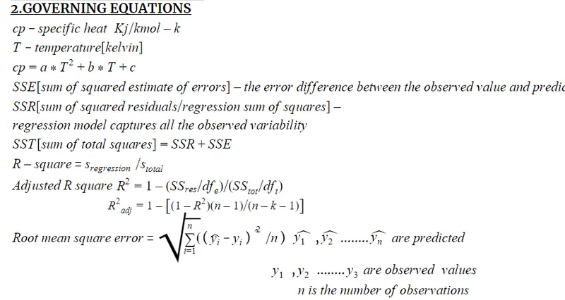
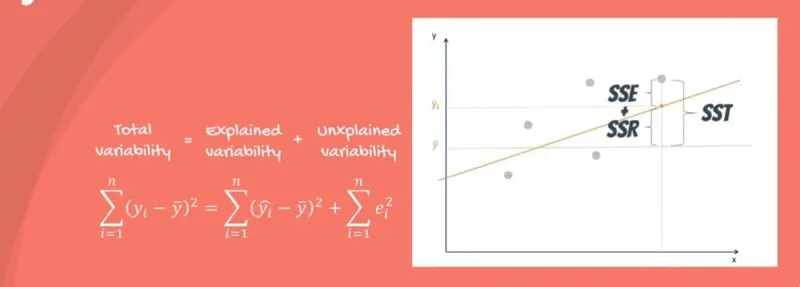
SST- The sum of squares total, denoted SST, is the squared differences between the observed dependent variable and its means
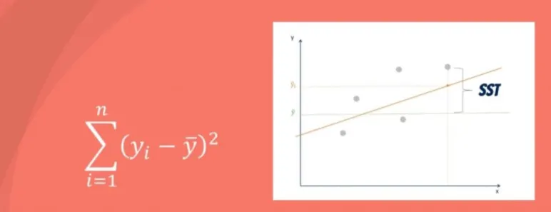
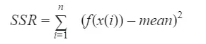
SSR sum of squares due to regression, or SSR. It is the sum of the differences between the predicted value and the mean of the dependent variable.
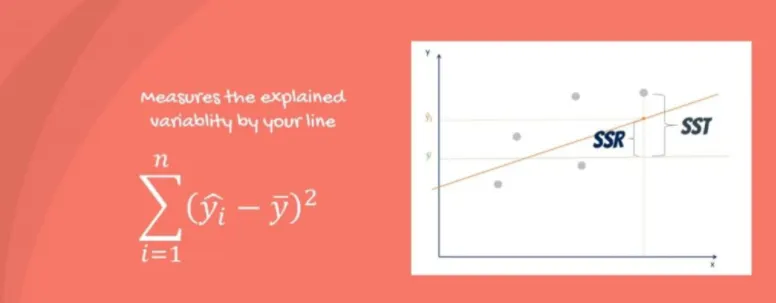
If this value of SSR is equal to the sum of squares total, it means our regression model captures all the observed variability and is perfect.
SSE [ sum of squares error]-The error is the difference between the observed value and the predicted value.To minimise The smaller the error, the better the estimation power of the regression. It is also known as RSS or residual sum of squares. Residual as in: remaining or unexplained.
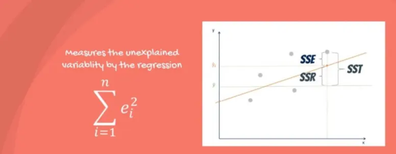
SST = SSR + SSE.
R-Squared (R² or the coefficient of determination) r-squared shows how well the data fit the regression model (the goodness of fit).The most common interpretation of r-squared is how well the regression model fits the observed data. Generally, a higher r-squared indicates a better fit for the model.Sometimes, a high r-squared can indicate the problems with the regression model.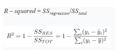
SSregression is the sum of squares due to regression (explained sum of squares)
SStotal is the total sum of squares[SST].
The sum of squares due to regression measures how well the regression model represents the data that were used for modeling. The total sum of squares measures the variation in the observed data (data used in regression modeling).
Adjusted R-Square-R2 shows how well terms (data points) fit a curve or line. Adjusted R2 also indicates how well terms fit a curve or line, but adjusts for the number of terms in a model. If you add more and more useless variables to a model, adjusted r-squared will decrease. ... n is the number of points in your data sample.

The RMSE is the square root of the variance of the residuals. It indicates the absolute fit of the model to the data–how close the observed data points are to the model's predicted values. Whereas R-squared is a relative measure of fit, RMSE is an absolute measure of fit.
RMSE=(SSE)/n
5.ALGORITHM
Step1; start the program
Step2;input commands to clear and close
Step3;use load command to load the data file that consists of the value of cp and temperature.assigned the values to a variable named cp_data.
Step4;using command temp=data (:,1) temperature values in first column are read
step5;cp=using command data(:,2)second column of cp values are read from data
Step6;code for curve fitting assigned
Step7;values of cp is find as a function of T .using an equation cp=a*T^2+b*T+c where a and b are coefficients,2 nd order
polynomial function of T.
Step8;use polyfit command is to find the coefficients a and b ,where
co_effs=polyfit(y,x,order of polynomial)
Step9;to determine the predicted values for specific heat use command polynomial value(polyval) and the read values assigned t predicted cp
Step10;use ‘plot’ command to plot the graph of predicted cp data and raw cp data
Step10;labelling commands are used to label x axis and y axis
xlabel(‘Temperature[k]’)
ylabel(‘specific heat[kj-mol/k]’)
Step11;use legend command is to differentiate the predicted data and raw data
Step12;give title to plot using command title(‘’)
Step13;find goodness of fit using SSE,SSR,SST ,R^2,RMSE
step14;error is the difference between cp and predicted cp
step15;SSE and sum is assigned to zero
Step16;for loop introduced from 1 to length of cp
i=1:length(cp)
step17; sse=sse+error(i)^2; sse=0 to length(cp) read by using loop command
Step18; sum of all cp value assigned to sum
Step19;n is no.of data which is length of cp
Step20;find out mean value by using equation sum/n
step21;SSR initialized from 0
step22;SSR =SSR+(predicted_cp(i)-mean)^2
Step23;find value of ssr to length of cp
step24;Find SST using equation,SST=SSR+SSE
Step25;find R square using r2=SSR/SST
Step26;find RMSE using equation RMSE=(SSE/n)^0.5
Step27;end the program
ALGORITHM FOR SPLIT WISE METHOD
step8;Find predicted cp value by assigning range of temperature and cp
Step9;plot them in figure1 using hold on command
step10;plot(predicted_cp,temp,’color’,’r’,’linewidth’,3)
step 11;plot raw cp -temperature data
Step12;end the program
6.PROGRAM FOR CUBIC POLYNOMIAL
clear all
close all
clc
cp_data=load('data');
temperature=cp_data(:,1)
cp=cp_data(:,2)
%curvefit
%cp=a*T^2+b*T+c
co_effs=polyfit(temperature,cp,3)
predicted_cp=polyval(co_effs,temperature);
%compare my curve fit with the original data
plot(temperature,cp,'linewidth',3)
hold on
plot(temperature,predicted_cp,'linewidth',3,'color','r')
xlabel('Temperature[k]')
ylabel('specific heat[kj/kmol-k]')
legend('original dataset','curvefit')
error=cp-predicted_cp;
%sse
sse=0
sum=0
for i=1:length(cp)
sse=sse+error(i)^2;
sum=sum+cp(i);
end
n=length(cp)
mean=sum/n
%ssr
ssr=0
for(j=1:length(predicted_cp));
ssr=ssr+(predicted_cp(i)-mean)^2;
end
%calculating sst
sst=ssr+sse;
%r^2
r2=(ssr/sst);
%rmse
rmse=(sse/n)^0.5;
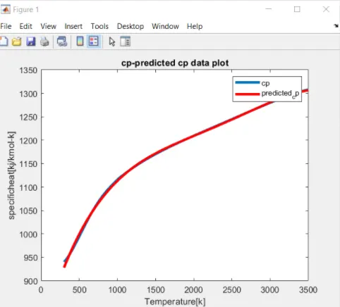
7.OUTPUT
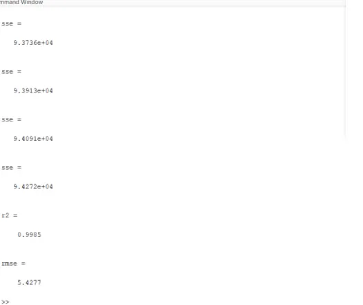
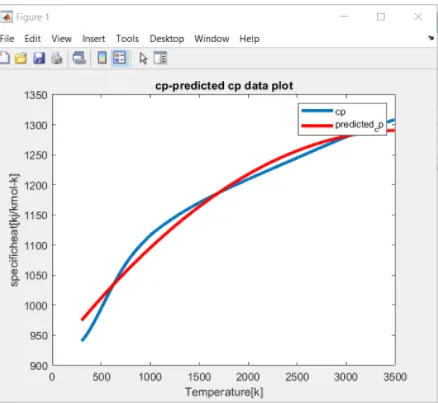
PROGRAM FOR SECOND DEGREE POLYNOMIAL
clear all
close all
clc
cp_data=load('data');
temperature=cp_data(:,1)
cp=cp_data(:,2)
%curvefit
%cp=a*T^2+b*T+c
co_effs=polyfit(temperature,cp,2)
predicted_cp=polyval(co_effs,temperature);
%compare my curve fit with the original data
plot(temperature,cp,'linewidth',3)
hold on
plot(temperature,predicted_cp,'linewidth',3,'color','r')
xlabel('Temperature[k]')
ylabel('specific heat[kj/kmol-k]')
legend('original dataset','curvefit')
error=cp-predicted_cp;
%sse
sse=0
sum=0
for i=1:length(cp)
sse=sse+error(i)^2;
sum=sum+cp(i);
end
n=length(cp)
mean=sum/n
%ssr
ssr=0
for(j=1:length(predicted_cp));
ssr=ssr+(predicted_cp(i)-mean)^2;
end
%calculating sst
sst=ssr+sse;
%r^2
r2=(ssr/sst);
%rmse
rmse=(sse/n)^0.5;

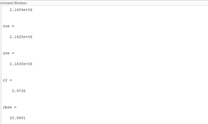
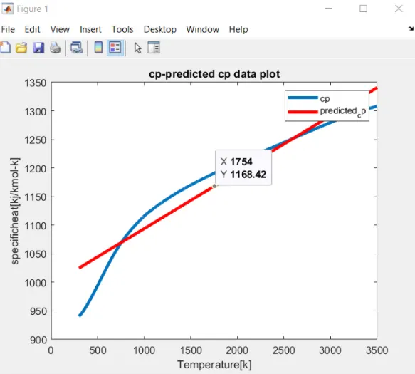
PROGRAM FOR LINEAR DEGREE POLYNOMIAL
clear all
close all
clc
cp_data=load('data');
temperature=cp_data(:,1)
cp=cp_data(:,2)
%curvefit
%cp=a*T^2+b*T+c
co_effs=polyfit(temperature,cp,1)
predicted_cp=polyval(co_effs,temperature);
%compare my curve fit with the original data
plot(temperature,cp,'linewidth',3)
hold on
plot(temperature,predicted_cp,'linewidth',3,'color','r')
xlabel('Temperature[k]')
ylabel('specific heat[kj/kmol-k]')
legend('original dataset','curvefit')
error=cp-predicted_cp;
%sse
sse=0
sum=0
for i=1:length(cp)
sse=sse+error(i)^2;
sum=sum+cp(i);
end
n=length(cp)
mean=sum/n
%ssr
ssr=0
for(j=1:length(predicted_cp));
ssr=ssr+(predicted_cp(i)-mean)^2;
end
%calculating sst
sst=ssr+sse;
%r^2
r2=(ssr/sst);
%rmse
rmse=(sse/n)^0.5;
OUTPUTS
8.USING ‘CFTOOL’
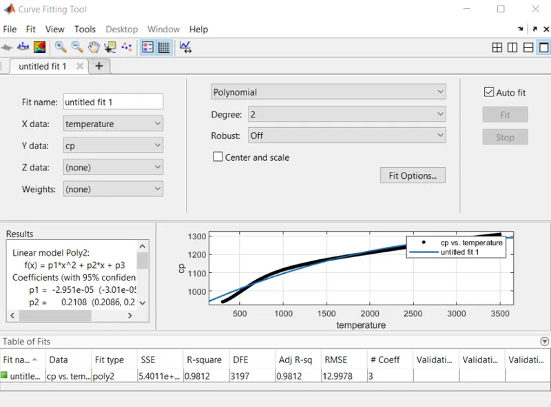
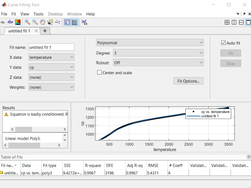
SPLIT WISE METHOD
clear all
close all
clc
%data
cp_data=load('data')
temp=cp_data(:,1);
cp=cp_data(:,2)
%curvefit
%cp=a*T^2+b*T+c
%splitting of data
temp1= cp_data(1:200,1);
temp2= cp_data(201:400,1);
temp3= cp_data(401:600,1);
temp4= cp_data (601:800,1);
temp5= cp_data(801:1000,1);
temp6=cp_data(1001:1200,1);
temp7=cp_data(1201:1400,1);
temp8=cp_data(1401:1600,1);
temp9=cp_data(1601:1800,1);
temp10=cp_data(1801:2000,1);
temp11=cp_data(2001:2200,1);
temp12=cp_data(2201:2400,1);
temp13=cp_data(2401:2600,1);
temp14=cp_data(2601:2800,1);
temp15=cp_data(2801:3000,1);
temp16=cp_data(3001:3200,1);
cp1= cp_data (1:200,2);
cp2= cp_data (201:400,2);
cp3= cp_data (401:600,2);
cp4= cp_data (601:800,2);
cp5= cp_data(801:1000,2);
cp6=cp_data (1001:1200,2);
cp7= cp_data(1201:1400,2);
cp8= cp_data(1401:1600,2);
cp9= cp_data(1601:1800,2);
cp10=cp_data(1801:2000,2);
cp11=cp_data(2001:2200,2);
cp12=cp_data(2201:2400,2);
cp13=cp_data(2401:2600,2);
cp14=cp_data(2601:2800,2);
cp15=cp_data(2801:3000,2);
cp16=cp_data(3001:3200,2);
co_effs_1=polyfit(temp1,cp1,2);
predicted_cp_1=polyval(co_effs_1,temp1);
co_effs_2=polyfit(temp2,cp2,2);
predicted_cp_2=polyval(co_effs_2,temp2);
co_effs_3=polyfit(temp3,cp3,2);
predicted_cp_3=polyval(co_effs_3,temp3);
co_effs_4=polyfit(temp4,cp4,2);
predicted_cp_4=polyval(co_effs_4,temp4);
co_effs_5=polyfit(temp5,cp5,2);
predicted_cp_5=polyval(co_effs_5,temp5);
co_effs_6=polyfit(temp6,cp6,2);
predicted_cp_6=polyval(co_effs_6,temp6);
co_effs_7=polyfit(temp7,cp7,2);
predicted_cp_7=polyval(co_effs_7,temp7);
co_effs_8=polyfit(temp8,cp8,2);
predicted_cp_8=polyval(co_effs_8,temp8);
co_effs_9=polyfit(temp9,cp9,2);
predicted_cp_9=polyval(co_effs_9,temp9);
co_effs_10=polyfit(temp10,cp10,2);
predicted_cp_10=polyval(co_effs_10,temp10);
co_effs_11=polyfit(temp11,cp11,2);
predicted_cp_11=polyval(co_effs_11,temp11);
co_effs_12=polyfit(temp12,cp12,2);
predicted_cp_12=polyval(co_effs_12,temp12);
co_effs_13=polyfit(temp13,cp13,2);
predicted_cp_13=polyval(co_effs_13,temp13);
co_effs_14=polyfit(temp14,cp14,2);
predicted_cp_14=polyval(co_effs_14,temp14);
co_effs_15=polyfit(temp15,cp15,2);
predicted_cp_15=polyval(co_effs_15,temp15);
co_effs_16=polyfit(temp16,cp16,2);
predicted_cp_16=polyval(co_effs_16,temp16);
plot(temp,cp,'linewidth',3);
hold on
plot(temp1,predicted_cp_1,'linewidth',3,'color','r');
plot(temp2,predicted_cp_2,'linewidth',3,'color','r');
plot(temp3,predicted_cp_3,'linewidth',3,'color','r');
plot(temp4,predicted_cp_4,'linewidth',3,'color','r');
plot(temp5,predicted_cp_5,'linewidth',3,'color','r')
plot(temp6,predicted_cp_6,'linewidth',3,'color','r')
plot(temp7,predicted_cp_7,'linewidth',3,'color','r')
plot(temp8,predicted_cp_8,'linewidth',3,'color','r');
plot(temp9,predicted_cp_9,'linewidth',3,'color','r');
plot(temp10,predicted_cp_10,'linewidth',3,'color','r');
plot(temp11,predicted_cp_11,'linewidth',3,'color','r');
plot(temp12,predicted_cp_12,'linewidth',3,'color','r');
plot(temp13,predicted_cp_13,'linewidth',3,'color','r');
plot(temp14,predicted_cp_14,'linewidth',3,'color','r');
plot(temp15,predicted_cp_15,'linewidth',3,'color','r');
plot(temp16,predicted_cp_16,'linewidth',3,'color','r');
title('cp-predicted cp data plot');
xlabel('Temperature[k]')
ylabel('specific heat[kj/kmol-k]')
legend('cp','predicted_cp')
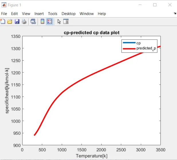
OUTPUT
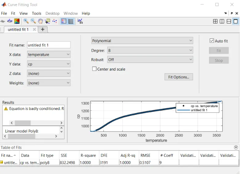
Mistakes and output
Badly conditioned" means that the solution of the system of linear equations critically depends on rounding errors due to the limited precision.
A valid solution (not a workaround only) is the scaling.
CONCLUSION
Perfect fit;It is phenomenon that each data point assigns with the polynomial function
Best fit;It is phenomenon that set of data is mapped as a polynomial function
Cubic fit;In order to fit the cubic polynomial data can be splitted into several intervals and polynomial function is computed
R square value for second degree polynomial is 0.9856 fit
R square value for cubic polynomial is 0.9985 fit.
R square value for linear polynomial is 0.9736 fit.
SSE,R Square,Adjusted R2,RMSE calculated.
The matlab program has been executed successfully and the output is verified
Question and answers
1.How to make a curfit perfectly?
Ans:The perfect fit is the fit where it should match the original curve and shouldn't have any scaling and centering error in that particular degree of the polynomial.The R^2 value must be 1 and SSEshould be 0.
2.how to get best fit?
ans:A perfect bit is an example of a best fit but all best fits are not perfect fit.
A best fit can be achived by
*As we increase the degree of a polynomial
*to use split wise data method(split x and y data into a equal range or folds and do the curve fitting)
3.what could be done to improve the cubic fit?
use split wise method ,split the data into smaller datasets and plot them
CODE
%curve fitting of linear polynomial
close all
clc

cp_data=load('data');
temperature=cp_data(:,1);
cp=cp_data(:,2);

%curvefit
%cp=a*T^2+b*T+c
co_effs=polyfit(temperature,cp,1)
predicted_cp=polyval(co_effs,temperature)

%compare my curve fit with the original data
plot(temperature,cp,'linewidth',3);
hold on
plot(temperature,predicted_cp,'linewidth',3,'color','r')
title('cp-predicted cp data plot');
xlabel('Temperature[k]')
ylabel('specificheat[kj/kmol-k]')
legend('cp','predicted_cp')
 %goodness of fit
 error=cp-predicted_cp;

%sse
sse=0
sum=0
for i=1:length(cp)
    sse=sse+error(i)^2
    sum=sum+cp(i);
end

n=length(cp);
mean=sum/n;
%ssr
ssr=0;
for(j=1:length(predicted_cp));
    ssr=ssr+(predicted_cp(i)-mean)^2;
end
%calculatind sst
sst=ssr+sse;

%r^2
r2=(ssr/sst)

%rmse
rmse=(sse/n)^0.5
%curve fitting of cubic polynomial
close all
clc

cp_data=load('data');
temperature=cp_data(:,1);
cp=cp_data(:,2);

%curvefit
%cp=a*T^2+b*T+c
co_effs=polyfit(temperature,cp,3)
predicted_cp=polyval(co_effs,temperature)

%compare my curve fit with the original data
plot(temperature,cp,'linewidth',3);
hold on
plot(temperature,predicted_cp,'linewidth',3,'color','r')
title('cp-predicted cp data plot');
xlabel('Temperature[k]')
ylabel('specificheat[kj/kmol-k]')
legend('cp','predicted_cp')
 %goodness of fit
 error=cp-predicted_cp;

%sse
sse=0
sum=0
for i=1:length(cp)
    sse=sse+error(i)^2
    sum=sum+cp(i);
end

n=length(cp);
mean=sum/n;
%ssr
ssr=0;
for(j=1:length(predicted_cp));
    ssr=ssr+(predicted_cp(i)-mean)^2;
end
%calculatind sst
sst=ssr+sse;

%r^2
r2=(ssr/sst)

%rmse
rmse=(sse/n)^0.5
%spilt wise method

clear all
close all
clc
%data
cp_data=load('data')
temp=cp_data(:,1);
cp=cp_data(:,2)
%curvefit
%cp=a*T^2+b*T+c
%splitting of data
temp1=    cp_data(1:200,1);
temp2=  cp_data(201:400,1);
temp3=  cp_data(401:600,1);
temp4= cp_data (601:800,1);
temp5= cp_data(801:1000,1);
temp6=cp_data(1001:1200,1);
temp7=cp_data(1201:1400,1);
temp8=cp_data(1401:1600,1);
temp9=cp_data(1601:1800,1);
temp10=cp_data(1801:2000,1);
temp11=cp_data(2001:2200,1);
temp12=cp_data(2201:2400,1);
temp13=cp_data(2401:2600,1);
temp14=cp_data(2601:2800,1);
temp15=cp_data(2801:3000,1);
temp16=cp_data(3001:3200,1);

cp1=   cp_data (1:200,2);
cp2=  cp_data (201:400,2);
cp3=  cp_data (401:600,2);
cp4=  cp_data (601:800,2);
cp5=  cp_data(801:1000,2);
cp6=cp_data (1001:1200,2);
cp7= cp_data(1201:1400,2);
cp8= cp_data(1401:1600,2);
cp9= cp_data(1601:1800,2);
cp10=cp_data(1801:2000,2);
cp11=cp_data(2001:2200,2);
cp12=cp_data(2201:2400,2);
cp13=cp_data(2401:2600,2);
cp14=cp_data(2601:2800,2);
cp15=cp_data(2801:3000,2);
cp16=cp_data(3001:3200,2);


co_effs_1=polyfit(temp1,cp1,2);
predicted_cp_1=polyval(co_effs_1,temp1);

co_effs_2=polyfit(temp2,cp2,2);
predicted_cp_2=polyval(co_effs_2,temp2);

co_effs_3=polyfit(temp3,cp3,2);
predicted_cp_3=polyval(co_effs_3,temp3);

co_effs_4=polyfit(temp4,cp4,2);
predicted_cp_4=polyval(co_effs_4,temp4);

co_effs_5=polyfit(temp5,cp5,2);
predicted_cp_5=polyval(co_effs_5,temp5);

co_effs_6=polyfit(temp6,cp6,2);
predicted_cp_6=polyval(co_effs_6,temp6);

co_effs_7=polyfit(temp7,cp7,2);
predicted_cp_7=polyval(co_effs_7,temp7);

co_effs_8=polyfit(temp8,cp8,2);
predicted_cp_8=polyval(co_effs_8,temp8);

co_effs_9=polyfit(temp9,cp9,2);
predicted_cp_9=polyval(co_effs_9,temp9);

co_effs_10=polyfit(temp10,cp10,2);
predicted_cp_10=polyval(co_effs_10,temp10);

co_effs_11=polyfit(temp11,cp11,2);
predicted_cp_11=polyval(co_effs_11,temp11);

co_effs_12=polyfit(temp12,cp12,2);
predicted_cp_12=polyval(co_effs_12,temp12);

co_effs_13=polyfit(temp13,cp13,2);
predicted_cp_13=polyval(co_effs_13,temp13);

co_effs_14=polyfit(temp14,cp14,2);
predicted_cp_14=polyval(co_effs_14,temp14);

co_effs_15=polyfit(temp15,cp15,2);
predicted_cp_15=polyval(co_effs_15,temp15);

co_effs_16=polyfit(temp16,cp16,2);
predicted_cp_16=polyval(co_effs_16,temp16);


plot(temp,cp,'linewidth',3);
hold on
plot(temp1,predicted_cp_1,'linewidth',3,'color','r');
plot(temp2,predicted_cp_2,'linewidth',3,'color','r');
plot(temp3,predicted_cp_3,'linewidth',3,'color','r');
plot(temp4,predicted_cp_4,'linewidth',3,'color','r');
plot(temp5,predicted_cp_5,'linewidth',3,'color','r')
plot(temp6,predicted_cp_6,'linewidth',3,'color','r')
plot(temp7,predicted_cp_7,'linewidth',3,'color','r')
plot(temp8,predicted_cp_8,'linewidth',3,'color','r');
plot(temp9,predicted_cp_9,'linewidth',3,'color','r');
plot(temp10,predicted_cp_10,'linewidth',3,'color','r');
plot(temp11,predicted_cp_11,'linewidth',3,'color','r');
plot(temp12,predicted_cp_12,'linewidth',3,'color','r');
plot(temp13,predicted_cp_13,'linewidth',3,'color','r');
plot(temp14,predicted_cp_14,'linewidth',3,'color','r');
plot(temp15,predicted_cp_15,'linewidth',3,'color','r');
plot(temp16,predicted_cp_16,'linewidth',3,'color','r');
title('cp-predicted cp data plot');
xlabel('Temperature[k]')
ylabel('specificheat[kj/kmol-k]')
legend('cp','predicted_cp')