Curve fitting PYTHON
AIM
To determine the code to fit a linear and cubic polynomial for the Cp data.
Explanation
Curve fitting is the process of constructing a curve, or mathematical functions, which possess the closest proximity to the real series of data. By curve fitting, we can mathematically construct the functional relationship between the observed data set and parameter values etc,.
The accuracy of the curve fit can be improved by increasing the degree of polynomial. So, a best fit can obtained by increasing the degree of the polynomial
RMSE:
It stands for Root Mean Square Error. It equates to the square root of the squares of the sum of differences between each observed data value and the predicted value. The minimum value of the RMSE is the best for the best fit line. Basically, it is the square root of variance.
In other words, it is the standard deviation of the predicted values. It is a parameter to measure the distance between the data point and the regression line. It measures how spread out these residuals are. In simple words, we can say that it tells us how distributed the data is around the line of best fit.
R-squared (R²):
It measures the proportion of the variation in our dependent variable vis-a-vis the independent variables in the model.
It assumes that every independent variable in the model helps to explain variation in the dependent variable. In reality, some independent variables (predictors) don't help to explain the dependent (target) variable.
In other words, some variables do not contribute to predicting the target variable.
Mathematically, we can calculate it by dividing the sum of squares of residuals (SSres) by the total sum of squares (SStot) and then subtract it from 1.
In this case, SStot measures the total variation. Ssreg measures explained variation and SSres measures the unexplained variation.
As SSres + SSreg = SStot,
R² = Explained variation / Total Variation
R-Squared is also called the coefficient of determination. It lies between 0% and 100%.
An r-squared value of 100% means the model explains all the variation of the target variable. And a value of 0% measures zero predictive power of the model.
So, the higher the R-squared value, the better the model.
Adjusted R-Squared:
The Adjusted R-Squared measures the proportion of variation explained by only those independent variables that really help in explaining the dependent variable.
It penalizes us for adding an independent variable that does not help in predicting the dependent variable.
Mathematically we can write it in the following manner:
Difference between R-squared and adjusted R-square:
1. Adjusted R-square can be negative only when R-square is very close to zero.
2. Adjusted R-Square values are always less than or equal to R-square but never be greater than R-Square.
3. If we add an independent variable to a model every time then, the R-squared increases, despite the independent variable being insignificant. This means that the R-square value increases when an independent variable is added despite its significance. Adjusted R-squared increases only when the independent variable is significant and affects the dependent variable.
Here we can see the formula of RMSE once again.
SSE is the sum of the squared differences between each observation and its group's mean. It can be used as a measure of variation within a cluster. If all cases within a cluster are identical the SSE would then be equal to 0.
The formula for SSE is:
1.
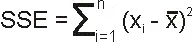
Where n is the number of observations xi is the value of the ith observation and 0 is the mean of all the observations. This can also be rearranged to be written as seen in J.H. Ward's paper.
2.
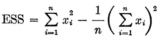
At each stage of cluster analysis the total SSE is minimized with SSEtotal = SSE1 + SSE2 + SSE3 + SSE4 .... + SSEn. At the initial stage when each case is its own cluster this of course will be 0.
import math
import matplotlib.pyplot as plt
import numpy as np
from scipy.optimize import curve_fit

#curve fit function
#Linear function

def function(t,a,b):
	return a*t + b


file = open('data', 'r')
def read_file():
	temperature = []
	cp = []

	for line in file:
		values =  line.split(',')
		temperature.append(float(values[0]))
		cp.append(float(values[1]))

	return [temperature,cp]


temperature,cp = read_file()
popt,pcov = curve_fit(function,temperature,cp)
fit_cp = function(np.array(temperature), *popt)

plt.plot(temperature,cp,'k--')
plt.plot(temperature,fit_cp, linewidth=2,color = 'red')
plt.xlabel('Temperature in K')
plt.ylabel('Heat')
plt.legend(['original dataset','linear polynomial'])
plt.title('linear polynomial')
plt.grid()
plt.savefig('linear fit')
plt.show()


#case 2 cubic polynomial

def function(t,a,b,c,d):
	return a*pow(t,3) + b*pow(t,2) + c*t + d


file = open('data','r')

def read_file():
	temperature = []
	cp = []


	for line in file:
		values = line.split(',')
		temperature.append(float(values[0]))
		cp.append(float(values[1]))

	return[temperature,cp]


temperature,cp = read_file()

popt,pcov = curve_fit(function,temperature,cp)
fit_cp = function(np.array(temperature),*popt)

plt.plot(temperature,cp,'k--')
plt.plot(temperature,fit_cp, linewidth = 2, color = 'magenta')
plt.legend('Temperature' ,'cp')
plt.legend(['original data','cubic_polynomial'])
plt.xlabel('Temperature in K')
plt.ylabel('Heat')
plt.title('cubic_polynomial')
plt.grid()
plt.savefig('cubic_fit')
plt.show()
OUTPUTS
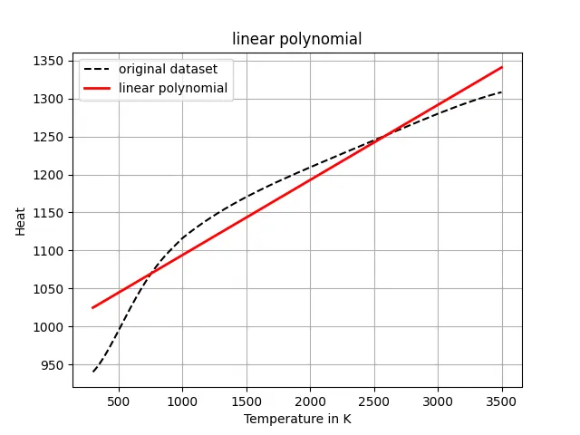
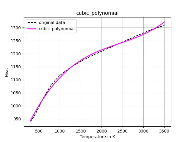
CUBIC POLYNOMIAL
A cubic polynomial is a polynomial of degree three, i.e., the highest exponent of the variable is three. A cubic polynomial, in general, will be of the form p(x): ax3 + bx2 + cx + d, a≠0
Given below are a few examples of cubic polynomials:
- p(x): x3 − 6x2 + 11x − 6
- q(y): 27y3 − 1
- r(z): πz3 + (√2)10
We observe that a cubic polynomial can have at the most four terms. Once again, the constraint that a should not be equal to 0 is required because if a is 0, then this becomes a quadratic rather than a cubic polynomial.
CODE EXPLANATION
Data file should be on same folder as the python file registry. The file containing data is copied to variable in the python program then we have the equations.
Import the required libraries
After that define the functions that are programmed to accept the values of t,a,b,c,d and return the value after calculating them all in cubic and linear equation respectively.
The cuve_fit function is used for both linear and cubic polynomials.
popt and pcov are the outputs of the function 'curve_fit'.
popt is the array that contains the optimal parameters or values of the coefficients
pcov is a 2D array that contains the estimated covariance of the parameters in popt.
popt and pcov values are found using curve_fir function.
The new values of specific heat are obtained by passing the obtained values form curve_fit to the defined functions.
1. What does popt and pcov mean?
popt and pcov are the output functions curve_fit. popt is the array that contains the optimal parameters or the values of the coefficient of the cubic equation. pcov is 2D array that contains the estimated co variance of the parametets in popt.
2. what does np.array(temperature) do?
np.array() is used to create a numpy array and the temperature is passed as the data of the array. Numpy array is a central data structure of the numpy library, which is a numerical library of python.
3.what does the *in* popt mean?
'*popt' is used to expand the list of values stores in the array 'popt; into the arguments of the function.
4.what needs to be done in order to make the curve fit perfect?
the order of the polynomial can be increased to obtain better results on curve fit as executed.