Week 5 - Curve fitting

1.AIM: to create a create fit function which best represents the given data.

2.GOVERNING EQUATIONS:

Curve fitting is the process of constructing a curve, or mathematical function, that has the best fit to a series of data points

• Quadratic equation: `ax^2+bx+c`
• Cubic equation:`ax^3+bx^2+cx+d`
• Quadratic equation:`ax^4+bx^3+cx^2+dx+e`

3.OBJECTIVES OF THE PROJECT:

1. What does popt and pcov mean?

- popt is an array of coefficients of polynomial specified at the beginning. pcov is a square matrix that contains the true variance and covariance of the parameters.

2. What does np.array(temperature) do?

- It creates an array of temperatures from the values in 'data file' using numpy module.

3. What does the * in *popt mean?

-It refers to the coefficients of the polynomial.

4. Write code to fit a linear and cubic polynomial for the Cp data. Explain if your results are good or bad.

5. What needs to be done in order to make the curve fit perfect?

-the value of RMSE should be minimum and the value of R² should be close to 1.

6. Show empirically as to how well your curve has been fit.

4.BODY OF THE CONTENT:

import the basic modules

create a function to the data file, create empty arrays for temp and cp. open the data file to read and split it and append the values of temp and cp as float. after that we return the values

in the main program we create a curve fit for a linear eq.

then we use the curve fit function in scipy module which contains the linear eq., temperature and specific heat.

we get 2 outputs popt and pocv, we then take the fun. and pass the temperature as numpy array along with copt which contains our variables.

when we get the curve fit we have to calculate the specific heat and its called as fit_cp.

then we create 2 plots one with temperature and cp and other with temperature and fit_cp

if the curve fit is perfect then both these curve should match.

import math
import matplotlib.pyplot as plt
import numpy as np
from scipy.optimize import curve_fit

#curve fit function
def fun(t,a,b):
	return a*t+b  #one dimensional equation to show relationshp betwen temperature and specific heat

# reading data file
def read():
	 t=[]
	 cp=[]
	 for line in open('data','r'):
	 	values=line.split(',')
	 	t.append(float(values[0]))
	 	cp.append(float(values[1]))
	 return[t,cp]	

#main program
t,cp=read()
popt,pcov=curve_fit(fun,t,cp)
fit_cp=fun(np.array(t),*popt)

plt.plot(t,cp,color="blue",linewidth=3)
plt.plot(t,fit_cp,color='red',linewidth=3)
plt.legend(['áctual data','çurve fit'])
plt.xlabel('temperature[K]')
plt.ylabel('Çp')
plt.title('Linear curve fit')
plt.show()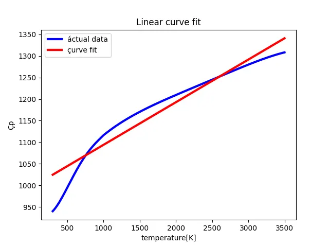	 	

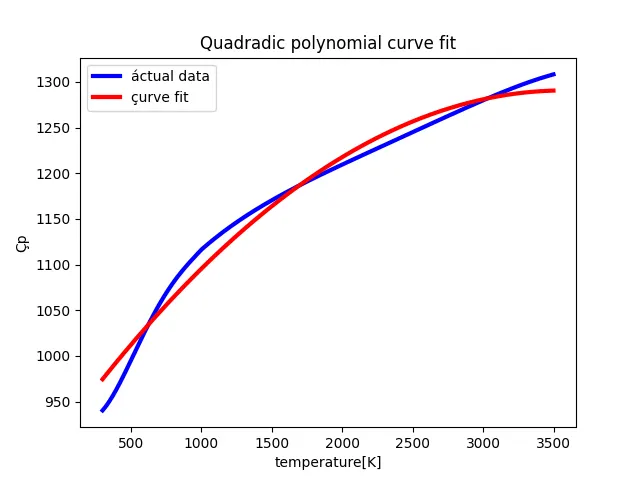
similarly for quadratic equation.

import math
import matplotlib.pyplot as plt
import numpy as np
from scipy.optimize import curve_fit

#curve fit function
def fun(t,a,b,c):
	return a*pow(t,2)+b*t+c  #quadratic equation to show relationshp betwen temperature and specific heat

# reading data file
def read():
	 t=[]
	 cp=[]
	 for line in open('data','r'):
	 	values=line.split(',')
	 	t.append(float(values[0]))
	 	cp.append(float(values[1]))
	 return[t,cp]	

#main program
t,cp=read()
popt,pcov=curve_fit(fun,t,cp)
fit_cp=fun(np.array(t),*popt)

plt.plot(t,cp,color="blue",linewidth=3)
plt.plot(t,fit_cp,color='red',linewidth=3)
plt.legend(['áctual data','çurve fit'])
plt.xlabel('temperature[K]')
plt.ylabel('Çp')
plt.title('Quadradic polynomial curve fit')
plt.show()	 	

we get the graph for linear and quadratic equations which shows us that the graph is not perfect, to improve the accuracy we need to use higher order functons.

similarly we create a curve for cubic polynomial.

import math
import matplotlib.pyplot as plt
import numpy as np
from scipy.optimize import curve_fit

#curve fit function
def fun(t,a,b,c,d):
	return a*pow(t,3)+b*pow(t,2)+c*t+d  #cubic equation to show relationshp betwen temperature and specific heat
	
# reading data file
def read():
	 t=[]
	 cp=[]
	 for line in open('data','r'):
	 	values=line.split(',')
	 	t.append(float(values[0]))
	 	cp.append(float(values[1]))
	 return[t,cp]	

#main program
t,cp=read()
popt,pcov=curve_fit(fun,t,cp)
fit_cp=fun(np.array(t),*popt)

plt.plot(t,cp,color="blue",linewidth=3)
plt.plot(t,fit_cp,color='red',linewidth=3)
plt.legend(['áctual data','çurve fit'])
plt.xlabel('temperature[K]')
plt.ylabel('Çp')
plt.title('cubic polynomial curve fit')
plt.show()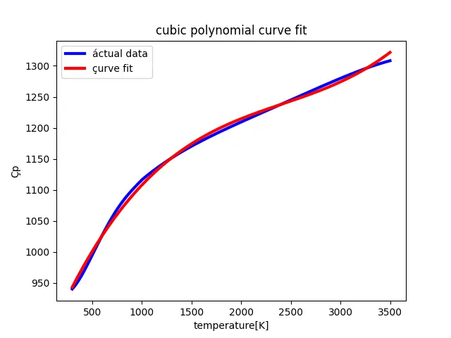	 	

from the graph we see that the accuracy increases but its not perfect to improve the accuracy we use a biquadratic equation.

import math
import matplotlib.pyplot as plt
import numpy as np
from scipy.optimize import curve_fit

#curve fit function
def fun(t,a,b,c,d,e):
	return a*pow(t,4)+b*pow(t,3)+c*pow(t,2)+d*t+e  #biquadratic equation to show relationshp betwen temperature and specific heat
	
# reading data file
def read():
	 t=[]
	 cp=[]
	 for line in open('data','r'):
	 	values=line.split(',')
	 	t.append(float(values[0]))
	 	cp.append(float(values[1]))
	 return[t,cp]	

#main program
t,cp=read()
popt,pcov=curve_fit(fun,t,cp)
fit_cp=fun(np.array(t),*popt)

plt.plot(t,cp,color="blue",linewidth=3)
plt.plot(t,fit_cp,color='red',linewidth=3)
plt.legend(['áctual data','çurve fit'])
plt.xlabel('temperature[K]')
plt.ylabel('Çp')
plt.title('biquadratic polynomial curve fit')
plt.show()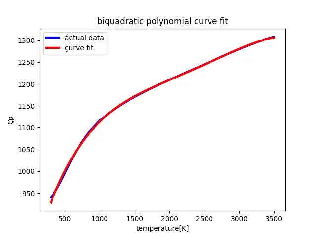	 	

from the graph the results are highly accurate as the order of polynomial increases.

5.CONCLUSION:

Curve Fitting of the given data is done by suitable methods in order to produce the best fit. The Linear and Quadratic Fit Curve doesn’t satisfy the criterion whereas Cubic and Biquadratic Fit Curve satisfies it.

For curve fitting plot we need three modules are numpy, matplotlib and scipy.

Different order equation has different curve fitting.

If order of equation is lesser then we get more error and bad curve fitting and vice versa.