Week 2 Air standard Cycle

MOHAMMED KHIZAR ALI ANSARI, MECH-A

1602-18-736-027

1.AIM: to create an otto cycle and plot it

2.GOVERNING law:

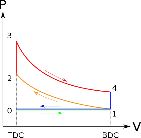
An Otto cycle is an idealized thermodynamic cycle that describes the functioning of a typical spark ignition piston engine. It is the thermodynamic cycle most commonly found in automobile engines. Otto cycle consists of two isoentropic and two isochoric processes. Engines operating under the Otto cycle are relatively inexpensive to manufacture and provide reasonable power to weight ratios with good efficiencies.

3.OBJECTIVES OF THE PROJECT:

to use python to:

1. create a PV diagram

2. output the thermal efficiency of the engine.

4.BODY OF THE CONTENT:

a function called engine is created which contains the variables- bore, stroke, conrod, start crank, end crank

parametres for all the states are found and written

based on these parameters we can calculate the swept volume and clearance volume.

`Vs=pi/4*b^2*s`

`Vc=(Vs) /(Cr-1)`

volume at state 1 will be vs+vc

we use the fornula which describrs the relation between crank angle and volume inside combustion chamber.

`V/(Vc)=1+0.5(r-1)[R+1-costheta-(R^2-sin^2theta)^0.5]`

which is divided in 3 parts and combined.

the start crank and end crank value will be defined

dheta is the crank angle spacing and numv is the number of values.

import math
import matplotlib.pyplot as plt

def engine(b,s,c,CR,s_c,e_c):
	pass
	
	a=s/2
	r=c/a

	#volume
	sv=(math.pi/4)*pow(b,2)*s
	cv=(sv)/(CR-1)
	v1=cv+sv

	sc=math.radians(s_c)
	ec=math.radians(e_c)

	numv=50
	dheta=(ec-sc)/(numv-1)

with this we can create and calculate the crank angle arrays and volume arrays using for loops which stores then in variable x&v

for state 2 the clearance vol. will be v2. for p2 we use the isentropic relation, `(p2*v2)^gamma=(p1*v1)^gamma`

using ideal gas law `(p1*v1)/(t1)=(p2*v2)/(t2)`

we know LHS and can define state 2 parameters and upto state 4

we call the function at state 2 to define the volume of compression from 180 to 0 (radians) using for loop and append

similarly we call the function at state 3 to define the volume of expansion from 0 to 180 (radians) using for loop and append

v=[]

	for x in range(0,numv):
		theta=sc+x*dheta
		term1=0.5*(CR-1)
		term2=r+1-math.cos(theta)
		term3=pow(r,2)-pow(math.sin(theta),2)
		term3=pow(term3,0.5)

		v.append((1+term1*(term2-term3))*cv)
	return v


#input parametres
p1=1000000
t1=373
b=0.2
s=0.3
c=0.5
CR=3	
g=1.4
t3=3000

#volume
sv=(math.pi/4)*pow(b,2)*s
cv=(sv)/(CR-1)
v1=cv+sv

#state2
v2=cv
p2=p1*pow(v1,g)/pow(v2,g)

#ideal law
rhs=p1*v1/t1	#this is constant
t2= p2*v2/rhs

v_comp=engine(b,s,c,CR,180,0)
constant=p1*pow(v1,g)

p_comp=[]

for y in v_comp:
	p_comp.append(constant/pow(y,g))

#state3
v3=v2 	#isochoric
rhs=p2*v2/t2
p3=rhs*t3/v3

v_exp=engine(b,s,c,CR,0,180)
constant=p3*pow(v3,g)

p_exp=[]

for y in v_exp:
	p_exp.append(constant/pow(y,g))

#state4
v4=v1 	#isochoric
p4=p3*pow(v3,g)/pow(v4,g)
t4=p4*v4/rhs

finally we create the state plots and plot for compression volume and compression pressure

label x&y axis as pressure and volume

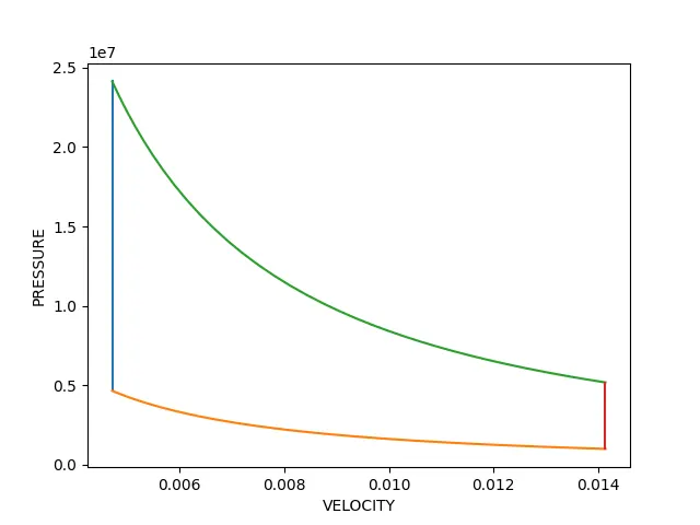
plt.plot([v2,v3],[p2,p3])
plt.plot(v_comp,p_comp)
plt.plot(v_exp,p_exp)
plt.plot([v4,v1],[p4,p1])
plt.xlabel('VELOCITY')
plt.ylabel('PRESSURE')
plt.show()

we get the plot as

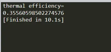
for calculating thermal efficiency we use the formula:`1-(1/(compression ratio)^(gamma-1))`

#thermal efficiency
part1=pow(CR,g-1)
efficiency=1-(1/part1)
print('thermal efficiency:')
print(efficiency)

the result we get

5.CONCLUSION:

when the function is called make sure that the order in which the parameters are passed are the same.

becareful with indendations.

when copying be careful with the code.