Basics of ML & AL Week 2 Challenge

Calculate all 4 business moments using pen and paper for the below data set?

1.First Business Moment - Mean

`μ = ∑ ( ( X i ) *P ( X ) )`

μ=(0⋅0.35)+(1⋅0.25)+(2⋅0.15)+(3⋅0.15)+(4⋅0.10)μ=(0⋅0.35)+(1⋅0.25)+(2⋅0.15)+(3⋅0.15)+(4⋅0.10)

μ=1.4

2.Second Business Moment - Variance

`σ^ 2 = ∑ ( ( X i − μ x )^ 2 ⋅ P ( X ) )`

`σ^2`=(0−1.4)2⋅0.35+(1−1.4)2⋅0.25+(2−1.4)2⋅0.15+(3−1.4)2⋅0.15+(4−1.4)2⋅0.10σ2=(0-1.4)2⋅0.35+(1-1.4)2⋅0.25+(2-1.4)2⋅0.15+(3-1.4)2⋅0.15+(4-1.4)2⋅0.10

`σ^2`=0.686+0.04+0.054+0.384+0.676σ2=0.686+0.04+0.054+0.384+0.676

`σ^2`=1.84

3. Third Business Moment - Skewness

`Sk = ∑ ( ( X i − μx) / σ )^ 3 ⋅ P ( X )`

We need to find the standard deviation, σσ using the variance value. The standard deviation is the square root of the variance:

standard deviaton,σ=1.36

substituting in the above formula,

Sk = (−0.38)+(−0.006)+0.0129+0.2442+0.6987(-0.38)+(-0.006)+0.0129+0.2442+0.6987

Sk = 0.57

4.Fourth Business Moment - Kurtosis

`Kt = ∑ (( X i − μx )/ σ )^ 4 ⋅ P ( X ) − 3`

substituting the variables in the formula

Kt = (0.393+0.00187+0.00568+0.287+1.3358)−3(0.393+0.00187+0.00568+0.287+1.3358)-3

Kt = -0.98

What is the significance of expected value when simple mean (Sum of all observations/number of observations) is already in place

Expected value is a theoretical value that shows the average return of an action you’d get if it was repeated infinite times. You can calculate expected value as the weighted average of all the possible outcome values — where the weight is the probability of the given outcome.

In Probability theory, the expected value of a random variable is the value you would expect to obtain if the random variable process was repeated for an infinite number of times and the average of those values were taken.

The mean of a data set is exactly the same by definition and concept as the expectation and mainly differs in application. When we have a data set along with its frequencies, then we use the mean formula to calculate the average. By summing up the product of the random variable with its frequency and dividing by the total frequency, we get the average value. If instead, we had a data set with the probabilities of occurrence for each random variable, then we would use the expectation formula to determine the average. Also, if the probabilities for all of the random variables are equal, then we can find the average using the mean directly instead of the expectation. Both are the same conceptually because the frequency of a variable occurring is the same as its probability of occurrence.

You have two outcomes: heads or tails. The probabilities of both are 50%.Let’s say that you play 100 rounds with your friend. You risk $1 in each round. If it’s tails, you double your money, if it’s heads, you lose your money.The expected revenue from this game is $1. And you have to invest $1 in each round. So your expected value of your profit is $0. In other words, if you play this game long enough, you won’t lose or win any money.

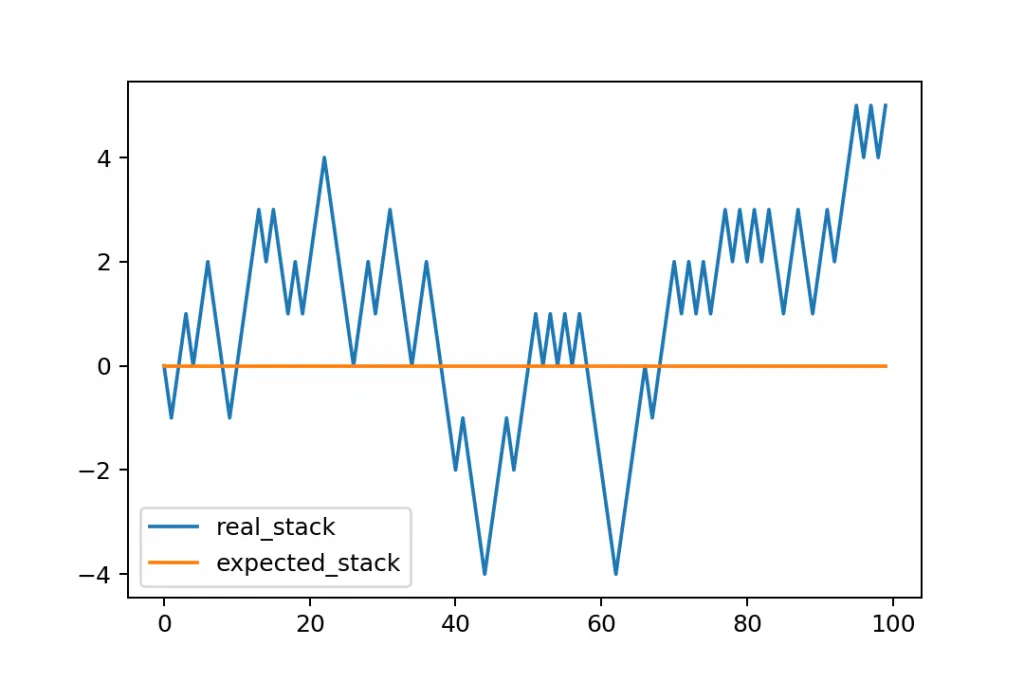
• The orange line represents the expected value in each round. This is the theoretical value. Luck is eliminated. Again, it’s always $0 because your investment ($1) equals your expected revenue ($1).
• The blue line is the real stack. It has a natural variance. It goes up and down, depending whether you were lucky (you got heads) or unlucky (you got tails).
• As you can see, the expected value was $0 – but you ended up with $5 after all. Yeah, this happens, you know, it’s called blind luck. But calculating the expected value helps rationalize that

Is having skewness in the curve considered to be bad in the analysis?

Skewness refers to distortion or asymmetry in a symmetrical bell curve, or normal distribution, in a set of data. If the curve is shifted to the left or to the right, it is said to be skewed. It measures the lack of symmetry in data distribution.It differentiates extreme values in one versus the other tail.

Let us take a very common example of house prices. Suppose we have house values ranging from $100k to $1,000,000 with the average being $500,000.

If the peak of the distribution was left of the average value, portraying a positive skewness in the distribution. It would mean that many houses were being sold for less than the average value, i.e. $500k. This could be for many reasons, but we are not going to interpret those reasons here.

If the peak of the distributed data was right of the average value, that would mean a negative skew. This would mean that the houses were being sold for more than the average value.

having skewness in data can be either bad or good it depends on type of analysis we are going to perform.

Evaluate the probabilities for continuous normal distribution with given mean = 680 and standard deviation = 31

a)P(X<711)

b)P(X>740)

c)P(600<X<720)

d)P(X=720)

`z = (x − μ)/ σ`

Where, x is the random variable

μ=Mean

σ=Standard deviation

a. x=711 importing it in the formula,z=1

Using the Z-score tables, find the corresponding probability for P(Z < 1 )

P(Z < 1) = 0.8413 (this is the area to the left of the z score, since we are finding the probability for x less than 711)

b) x=740; z=1.935

Using the Z-score tables, find the corresponding probability for P(Z < 1.935)

P(Z < 1.935) = 0.9713 (this is the area to the left of the z score)

We need to find the area to the right of the z - score, because we need the area for when X is greater than 740. So we need to subtract the left score from 1.

P (Z > 1.935) = 1 - P(Z < 1.935)

P (Z > 1.935) = 1 - 0.9713

P (Z > 1.935) = 0.0287

c) x=600, 720

therefore z=−2.58 & 1.29 respectively

We need to find the area for the z score less than -2.58 and subtract this from the area of the z score less than 1.29:

P(-2.58 < Z < 1.29) = P(Z < 1.29) - P(Z < -2.58)

P(-2.58 < Z < 1.29) = 0.90320 - 0.00466

P(-2.58 < Z < 1.29) = 0.89854

d)x=720; z=1.29

We need to find the area at z = 1.29

P(Z = 1.29) = P(1.29 < Z < 1.29)

P(Z = 1.29) = P(Z < 1.29) - P(Z < 1.29)

P(Z = 1.29) = 0.9032 - 0.9032

therefore P(Z = 1.29) = 0.

Explain the curve on the right side.

The curve shows the normal distribution of a random variable. The percentages show the standard deviations from the central value(mean).

1 standard deviation from the mean is approximately 34.1% to either the left or the right side of the mean. This means that the standard deviation of a normal distribution can lie anywhere within the space of + or - 34.1%. So, approximately 68.2% of the values in the distribution fall within 1 standard deviation of the mean.

Similarly, beyond the first standard deviation, 13.6% to the left or to the right of the first standard deviation represent the values that fall within the second standard deviation. This means to say that 95.4% (34.1+34.1+13.6+13.6) of the values in the distribution fall within 2 standard deviations of the mean.

This continues to the third standard deviation and so on with the area under the curve increasing.

For an ideal normal distribution curve, it will have no skewness and so will have perfect symmetry.