Week 3 - Solving second order ODEs

MOHAMMED KHIZAR ALI ANSARI,MECH-A

1602-18-736-027

1.AIM:

to solve an ODE of a simple pendulum.

2.GOVERNING EQUATIONS

In Engineering, ODE is used to describe the transient behavior of a system. A simple example is a pendulum. it can also be used in spring, mass and damping system.

The way the pendulum moves depends on the Newtons second law. When this law is written down, we get a second order Ordinary Differential Equation that describes the position of the "ball" w.r.t time.

g = gravity in m/s2,

L = length of the pendulum in m,

m = mass of the ball in kg,

b=damping coefficient.

the mentioned formula is a second order ODE, we breakém to series of first order ODE's

`(d theta)/dt=(d theta1)/dt=theta2`

`(d^2 theta)/dt^2=(d^2 theta1)/dt^2=(d theta2)/dt`

by substituting these eqs in the formula, we get

`(d theta2)/dt+(b*theta2)/m+(g*sin theta1)/L=0`

the first ODE is:`(d theta1)/dt=theta2`

second ODE is:`(d theta2)/dt=-(b*theta2)/m-(g*sin theta1)/L`

3.OBJECTIVES OF THE PROJECT:

Write a program in Python that will simulate the pendulum motion

to create an animation

animate the motion of the pendulum

4.BODY OF THE CONTENT:

first we import the basic modules required.

next we import the variables:

l=1 metre,

m=1 kg,

b=0.05.

g=9.81 m/s2.

Simulate the motion between 0-20 sec, for angular displacement=0,angular velocity=3 rad/sec at time t=0.

we define the imitial condition for ODE which consists of an array of [displacement,velocity]

we then write a time array using the numpy module and linspace command. we start at 0 sec and integrate upto 10s and taking 200 values.

we then use an odeint command from the scipy module to solve and integrate ODE, which needs to contain a system,initial condition, time and arguments.

the system is a function which represents ODE. line 11&12 represent our 1st&2nd ODE and combine them into ODE called dheta_dt and theta will be the solution vector.

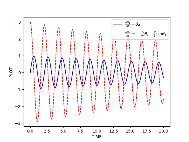
theta contains 2 columns- first for displacement(theta[:,0]) ODE second for velocity ODE (theta[:,1]).

import math
import matplotlib.pyplot as plt
import numpy as np
from scipy.integrate import odeint

def mod(theta,t,b,g,l,m):
	theta1=theta[0]
	theta2=theta[1]
	dheta1_dt=theta2
	dheta2_dt=-(b/m)*theta2-(g/1)*math.sin(theta1)
	dheta_dt=[dheta1_dt,dheta2_dt]
	return dheta_dt
	
#input variables	
l=1 
m=1 
b=0.05
g=9.81

#condition for first ODE [displacement,velocity]
theta0=[0,3]

#time arrays
t=np.linspace(0,20,200)

# to solve ODE
theta=odeint(mod,theta0,t,args=(b,g,l,m))

#plot
plt.plot(t,theta[:,0],'b-',label=r'$\frac{d\theta_1}{dt}=\theta2$')
plt.plot(t,theta[:,1],'r--',label=r'$\frac{d\theta2}{dt}=-\frac{b}{m}\theta_2-\frac{g}{L}sin\theta_1$')
plt.xlabel('TIME')
plt.ylabel('PLOT')
plt.legend(loc='best')
plt.show()

after plotting we note both displacement and velocity decreases due to dampening.

next we need to plot and create a pendulum with an animation by using for loops and ploting the dimensions of ball and rope.

taking linewidth = 15, markersize = 25 for ball at t=0s

create a grid and name the title as pendulum motion

#to plot and create a pendulum
ball_dis = theta[:,0]
count = 1
x0 = 0
y0 = 0
l = 3
for i in t:

    for x in ball_dis:
        pos_x = x0 +l*math.sin(math.radians(180) + x)
        pos_y = y0 +l*math.cos(math.radians(180) + x)

        filename = '%05d.png' % count
        count = count + 1
        plt.figure()
        plt.plot([-0.25,0.25],[0,0], linewidth = 15)
        plt.plot(x0,y0,marker ='*',markersize = 13)
        plt.plot([x0,pos_x],[y0,pos_y],linestyle ='-')
        plt.plot(pos_x,pos_y,'o',markersize = 25)
        plt.xlim([-4,4])
        plt.ylim([-5,1])
        plt.grid(True)
        plt.title('pendulum motion')
        plt.savefig(filename)

save as png and generate a gif from the images.

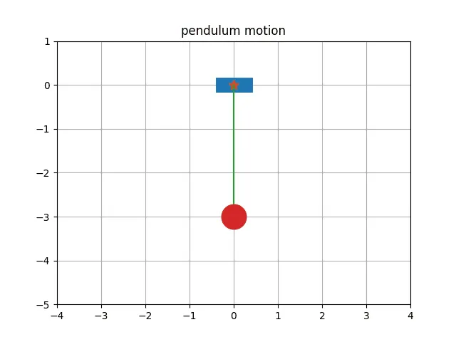(animation might stutter here but i have uploaded the proper animation at the end as gif)

5.CONCLUSION:

be careful with syntax.

use indendations appropriately.