Week 5.2 - Literature review: ODE Stability

AIM: To understand the importance of the stbaility analysis of ODE.

OBJECTIVES:

1. To find out when does ODE gets unstable
2. What is its effect o engineering solutions
3. Can stabilty condition be derived for all sort of problems and explain this theory prtaically with a python code.

INTRODUCTION:

An ODE is also known as the ordinary differential equation is a form differential equation that contains one or more functions of one independent variable. The solution of an ODE is a function that satisfies the equation. Finding an analytical solution of ODE is difficult for complex problems. So in such cases we perfom numerical solutions which could match the accuracy of the analytical solution.

One of the important characteristics of the solution algorithm is its stability. An algorithm or numerical scheme is said to be stable if, for a small change in the input, there must only be a small change in the output. In the numerical calculation process, small errors are introduced which can amplify as the solution marches in time and the result may blow up resulting in unphysical solutions.

An important aspect of ODEs is the condition of the expressions. If there is only a slight variation in the output for a slight variation in the input the expression is said to be well-conditioned. If there is a large variation in the output for a small variation in the input, the expression is said to be ill-conditioned.

It is also important to note that for a well-conditioned expression there is a stable way of solving and if the problem is ill-conditioned there is no reliable way to solve it.

THOERY OF SAMPLE CODE:

An ODE is selected for the study and the expression is kept as general as possible. The ODE used in the solution is gien below:

`(d y)/ (d t) + c y + e^( − t) = 0`

This can also be written as `(dy)/(dt)= f(t)`

where `f(t)=-cy-e^(-t)`

`(d y)/ (d t) = − c y − e^ (− t)`

The numerical solution can be done in two different ways, the explicit Eulers method and the implicit Eulers method.

The explicit Euler method uses the values from the previous time step to calculate the value in the current time step

`(y^(n+1)-y^n)/(Deltat)=-cy^n-e^-t`

`y^(n+1)=y^n+(-cy^n-e^-t)Deltat`

Where `y^(n+1)` is the current time step and `y^n` is the previous time step. It is interesting to note that the explicit method is not unconditionally stable. The stability of this method is highly dependent on the value of the time-step.

The implicit Euler method is shown below:

`(y^n-y^(n+1))/(Deltat)=-cy^n-e^-t`

`y^n=(-cy^n-e^-t)Deltat+y^(n-1)`

`y^n(1+cDeltat)+e^-tDeltat=y^(n-1)`

Therefore we can say

`y^n=(y^(n-1)-e^-tDeltat)/(1+cDeltat)`

For an initial value of `y(0)=0` we can derive the analytical solution as

`y=(e^(-ct)(1-e^((c-1)t)))/(c-1)`

The stability of the equation can be controlled using two parameters, the constant `c` and the time step `Deltat`.

CODE:

import matplotlib.pyplot as plt
import numpy as np


def explicit_euler(t_total,dt):
    t=np.arange(0,t_total,dt)
    y=np.zeros(len(t))
    for i in range(1,len(t)):
        y[i]=y[i-1]+dt*(-c*y[i-1]-np.exp(-t[i-1]))
    return [t,y]
    
def implicit_euler(t_total,dt):
    t=np.arange(0,t_total,dt)
    y=np.zeros(len(t))
    for i in range(1,len(t)):
        y[i]=(y[i-1]-np.exp(-t[i-1])*dt)/(1+c*dt)
    return [t,y]


        
def analytical_soln(t_total,dt):
    t=np.arange(0,t_total,dt)
    y=np.zeros(len(t))
    for i in range(1,len(t)):
        y[i]=(np.exp(-c*t[i])*(1-np.exp((c-1)*t[i])))/(c-1)
    return [t,y]

# Time known constrain
t_total=0.1
c=100
dt=1e-3

t,y_explicit=explicit_euler(t_total,dt)
t,y_implicit=implicit_euler(t_total,dt)
t,y_analytical=analytical_soln(t_total,dt)


plt.figure()
plt.plot(t,y_explicit,color='blue')
plt.plot(t,y_implicit,color='red')
plt.plot(t,y_analytical,color='orange')
plt.xlabel('Time (s)')
plt.ylabel('y')
plt.legend(['Explicit','Implicit','Analytical'])
plt.savefig('odestability.png')
plt.show()

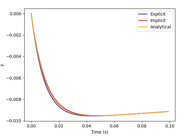
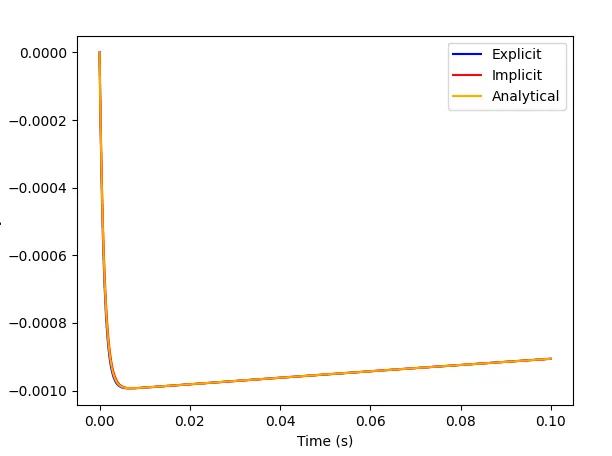
From the execution of the program, it is found that as the value of c increases, the time step needs to be decreased to get a stable solution.

It is found that when `c cdot dt= 0.1` there is an exact match between the explicit, implicit and analytical solution.

For c = 100 and dt = 1e-3 the solution plot is given below:

For c = 1000 and dt = 1e-4 the solution plot is given below:

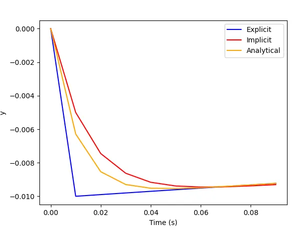
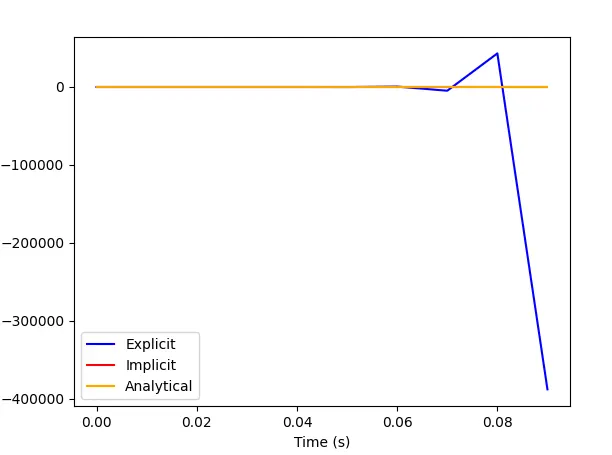
With increase in the time step the numerical solution starts devitating from the analytical solution.

For c = 100 and dt = 1e-2 the solution plot is given below:

For c = 1000 and dt = 1e-2 the solution plot is given below:

CONCLUSIONS:

From the detailed analysis of the ODE system, it is found that the constant c and time-step dt. It is found that if `c cdotdt=1.1`, the solution starts to become unstable.

It is also interesting to note that when `c cdot dt =0.1` the error is very less and the implicit and explicit schemes give almost the same result.

It is also found that the implicit scheme is stable irrespective of the time step in the differential equation considered in the above study. A generalization is not possible since in some cases there is a chance that the implicit scheme becomes unstable.

For different types of ODEs, the stability criterion will be different. If the criterion is not satisfied the solution becomes unstable.

An unstable solution implies that the solution is not physical and the results out of such simulation will not be realistic which cannot be used in engineering calculations.

From the literature review, it can be found out that the stability criteria can only be developed for well-conditioned equations. If the equation is ill-conditioned there is no reliable way for a stable solution.