Week 5.2 - Literature review: ODE Stability
Stability of ODE:
An ordinary differential equation has one independent variable and one or more orders of differential terms of the dependent variable with respect to the independent variable. In general, mathematical stability is defined such that when small pertubations are added to the independant variable, the function still converges to the actual solution rather than deviate from it. Often times numerical methods are preferred to obtain a solution for these ODE's due to the complex procedure to get analytical results, especially when the ODE's are complex. There are multiple numerical methods available for this purpose and choosing one of them requires the problem statement and their stability criteria. A numerical procedure generally has a numerical error due to the approximation made in the calculation. A numerical scheme is claimed to be stable when these errors reduce with each iteration and provide a convergent solution. The ODE scheme becomes unstable when the error tends to increase with each iteration and doens't converge towards the actual solution.
Lets consider a simple first order ODE in the generic form
`dy/dt = lambday`, where `lambda` -> arbitrary constant.
and derive the stability criteria for Euler(explicit) and Backward Euler(implicit) schemes to solve this ODE
Euler scheme (Explicit):
New values of y are calculated based on y values of previous iteration using first order Taylor approximation
`y_(n+1) = y_n + dy/dth = y_n + lambday_nh = y_n(1 + lambdah)`, where `h` -> step size
For each iteration, `y_(n+1)` is calculated as a function of `y_n` and for `y_(n+1)` to reach a converged solution, the term `(1 + lambdah)` should be less than 1.
`|1 + lambdah| < 1 => -1 < 1 + lambdah < 1 => -2 < lambdah < 0 `
Hence, `lambdah < 0` is the first condition for stability.
Since h is positive, `lambda` should be negative to obtain a stable solution.
For `lamda` being negative, `h < -2/lambda` is the second condition to achive stability while using explicit scheme.
Backward Euler (Implicit):
New values of y are calculated based on y values of current iteration using first order Taylor approximation
`y_(n+1) = y_n + dy/dth = y_n + lambday_(n+1)h`
`y_(n+1) - lambdahy_(n+1) = y_n`
`y_(n+1) = y_n(1/(1-lambdah))`
For this scheme to be stable, `|1/(1-lambdah)| < 1 => -1 < 1/(1-lambdah) < 1 => 1-lambdah > 1`
Hence, `lambdah < 0` is the stability criteria for implicit scheme.
Both schemes have `lambdah < 0` condition. When `lambda` is positive, both the schemes are unstable, meaning the numerical result for y in each step will diverge from the actual solution. Explicit sheme has an additional condition, `h < -2/lambda` that imposes a limit on the time-step size based on the lamda value.
Solving an ODE:
Lets take an acutual ODE, where y is a function of time t and h is the time-step size `Deltat` and try to solve it with the explicit and implicit schemes to check the stability criteria.
`dy/dt = -1000y - e^-t`, `y(t=0) = 0`
Comparing with generic ODE format and considering the effect of `e^-t` insignificant on stability, `lambda = -1000`. Since `lambda` is negative, the first condition of explicit scheme and the sole condition for implicit scheme is satisfied.
Using the explicit scheme,
`y_(n+1) = y_n + dy/dt*Deltat`
`y_(n+1) = y_n + (-1000*y_n - e^-t)*Deltat`
The second condition for explicit scheme is
`Deltat < -2/-1000 => Deltat < 0.002`
When this condition is satisfied, explicit scheme is stable.
Using implicit scheme,
`y_(n) = y_(n-1) + dy/dt*Deltat`
`y_(n) = (y_(n-1) - e^-t*Deltat)/(1+1000*Deltat)`
The implicit scheme is unconditionally stable since `lambda` is negative
Analytical solution:
The solution for differential equation obtained using online calculator is
`y = (e^(-1000 t) (1 - e^(999 t)))/999`
A python program is written to test out both these schemes and their stability criteria. The program solves for the differential equation provided using explicit, implicit and analytical methods for a range of dt values and compares them using xy plots
'''
Solve the equaiton `dy/dt = -1000y - e^-t`
using explicit and implicit schemes
and check the stability criteria
'''
import numpy as np
import matplotlib.pyplot as plt
import math

dt_arr = [0.0001, 0.001, 0.0019, 0.002, 0.01]  	# values of dt to be solved for
tmax = 0.1										# max value for t
t0 = 0											# min value for t
y0 = 0											# initial condition for y at t0

def explicit(y0,t_arr):
	# Solve the differential equation using explicit scheme
	y = y0
	y_arr = [y0]
	for t in t_arr[1:]:
		y = y + dt*(-1000*y - math.exp(-t))
		y_arr.append(y)
	return y_arr

def implicit(y0,t_arr):
	# Solve the differential equation using implicit scheme
	y = y0
	y_arr = [y]
	for t in t_arr[1:]:
		y = (y - math.exp(-t)*dt) / (1 + 1000*dt)
		y_arr.append(y)
	return y_arr

def analytical(y0,t_arr):
	# Solve the differential equation using implicit scheme
	y = y0
	y_arr = [y]
	for t in t_arr[1:]:
		y = (math.exp(-1000*t)*(1 - math.exp(999*t)))/999
		y_arr.append(y)
	return y_arr


for i in range(len(dt_arr)):
	# Solve y for given range of t and dt using all the schemes
	dt = dt_arr[i]
	t_arr = np.arange(t0,tmax,dt)
	y_exp_arr = explicit(y0, t_arr)
	y_imp_arr = implicit(y0, t_arr)
	y_anal = analytical(y0, t_arr)

	# plot y vs t for a range of dt
	plt.figure(i+1)
	plt.plot(t_arr,y_exp_arr, label="explicit")
	plt.plot(t_arr,y_imp_arr, label="implicit")
	plt.plot(t_arr,y_anal, label="analytical")
	plt.legend()
	plt.grid()
	plt.xlabel("time")
	plt.ylabel("y")
	plt.title("y vs time, dt = %0.4f" %dt)

plt.show()
Results:
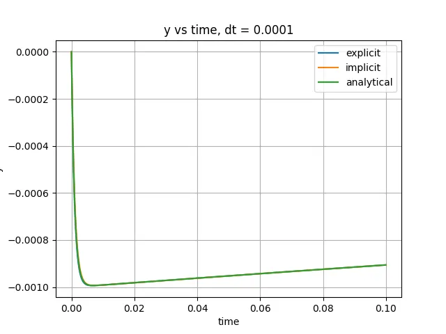
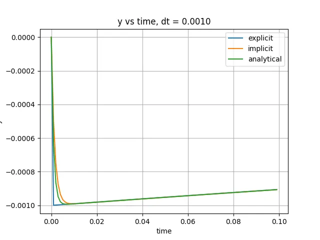
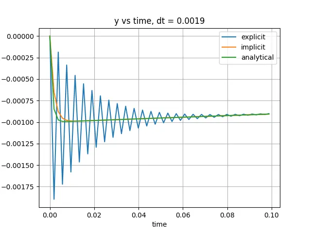
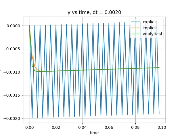
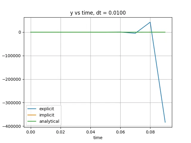
For a small value of dt such as 0.0001, compared to the explicit time-step limit of 0.002, both implicit and explicit schemes provide a very good approximation of y at all values of t. When dt is increased to 0.001, explicit scheme shows a large error near t=0, but the errors reduce over time and solution of y catches up with the analytical solution. Implicit scheme also shows error but smaller compared to explicit scheme near t=0 and similar to explicit, catches up with analytical results. With further increase in dt to 0.0019, a value very close to the time-step limit of explicit scheme, implicit scheme still shows the same behaviour as with previous time-step size. But explicit scheme seems to oscillate heavily near t=0. However, the amplitude of oscillations die down slowly so the y values reach the analytical solution at large values of t. Until now, both explicit and implicit schemes are considered stable since the error reduces over time to a solution that's close to actual solution. With dt taken as the same value of explicit time-step limit, 0.002, it can be seen that the osciallations for explicit scheme doesn't die down and seem to have a constant amplitude. This means even if the solution proceeds for a long duration, y value would never reach the actual solution, but remain at a constant error distance away from it. This behaviour is termed as neutrally stable condition, where the error doesn't increase or decrease with increasing time in the solution process. Above this limit, the solution using explicit scheme would become unstable. This is demonstrated with dt = 0.01 which shows y values go much farther than the actual solution with increasing t. So, the explicit scheme becomes unstable beyond dt values of 0.002. However the implicit scheme remains stable to predict correct values of y over larger t values with all the dt values chosen.
Stability in engineering simulations:
Stability is a major factor in engineering simulations, as it directly affects the error between the simulated results and actual results. Only if the simulation scheme is stable, would it be usefull to generate results that would pertain to physical meaning. An unstable scheme would constantly deviate from the physical result and the results would be unphysical and useless. Hence choosing a stable scheme is important in engineering applications to simulate a physical problem using numerical methods.
Stability of different problems:
Stability criteria can be obtained for almost all problems. There are multiple stability analysis schemes to analyse different problems. When a system of differential equation are involved with multiple variables forming coupled equations, a jacobian using first order derivaties are usually taken and evaluated at equilibrium points. When the real parts of all eigen values are negative, the ODEs are considered stable at that equilibrium point, otherwise unstable.