Week 5.2 - Literature review: ODE Stability

Stability of the ode

   we can say that the ode is stable if small changes in the initial condition of the ode does not affect the final solution of the ode.

   1)asymptotically stable

     

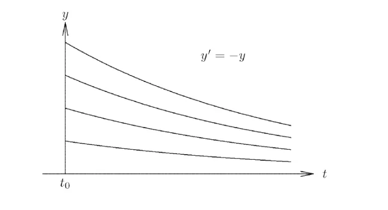
   from the figure we can see that no matter what is the value of y at t0 the solution is converging to the same value,than this ode is considerd as stable ode.

  2)unstable 

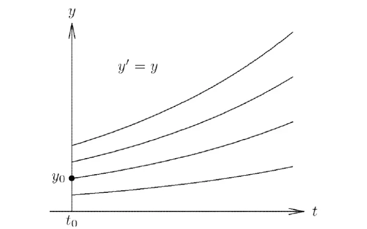
from the plot we can see that by changing the initial condition y0 the solution is diverging for each new condition than this ode is called unstable ode. 

Here we will look at the simple ode and see that for which method the solution of the ode is stable,

The ode is 

             `dy/dt=-2*y`

              now for this case 

              solution by the euler's forward difference 

                     `yn=yold+(dy/dt)*dt`

                           =`yold-2*yold*dt`

             solution by the euler's backward difference

                    `yn=yold+(dy/dt)*dt`

                    `yn=yold-2*yn*dt`

                    `yn+2*yn*dt=yold`

                     `(1+2*dt)yn=yold`

                   `yn=(yold)/(1+2*dt)`

             Analytical solution for this

                   `y=e^(-2*t+c)`

           here  for the stable solution we have to give initial condition as at t=0 ,y=1 so our c=0

                              we can not use the t=0 ,y=0 then it is critical point for the ode and solution is undefined

          Now for the stable solution of this problem our numerical method solution should go with the analytical solution and converging to the analytical solution as we move forward in                  time.

         PYTHON code file 

# ode stability 
""" solve the first order ode by explicit as well as implicit method to check the stability of the solution
ode is given by
               dy/dt=[-2*y]
               here the independent variable is t(time)
               dependent variable is y
               initial condition is at t=0 y=1
               time span is 0 to 2 seconds
"""

from cmath import exp
from tkinter import Y
from xml.dom.minidom import Element
import matplotlib.pyplot as plt
import numpy as np

# definig the time span for the solution
t=np.linspace(0,20,200)

# defining the time step size
dt=0.9

# defining the initial condition
y_0=1

# constant for the analytical solution for y_0=0 as initial condition
c=0


# defining the empty list for updating the solution at the end of iteratiion(analytical)
ya=[]

# defining the empty list for updating the solution at the end of iteration(explicit)
ye=[] 

# defining the empty list for updating the solution at the end of iteration(implicit)
yi=[]

# solve by the explicit method method
for i in t:
    ynew=y_0-2*y_0*dt
    y_0=ynew
    ye.append(y_0)

# solve by the implicit method method
for j in t:
    ynew=y_0/(1+2*dt)
    y_0=ynew
    yi.append(ynew)


# analytical solution
for i in t:
    ynew=1*exp(-2*i)
    y_0=ynew
    ya.append(y_0)

plt.plot(t,ye,color='red',linewidth='3',label='explicit method')
plt.plot(t,yi,color='blue',linewidth='3',label='implicit')
plt.plot(t,ya,color='black',linewidth='3',label='analytical')
plt.legend()
plt.xlabel('time')
plt.ylabel('Y')
title='time step size is:',(dt)
plt.title(title)
plt.show()

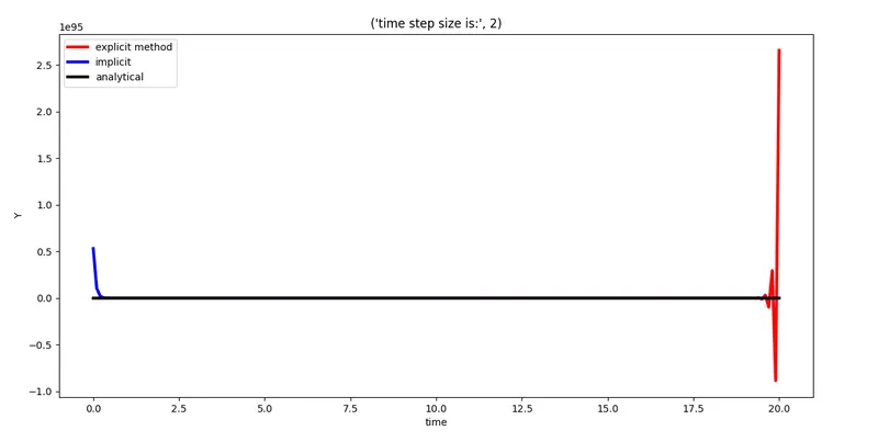
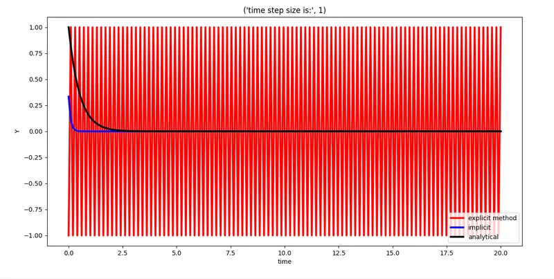
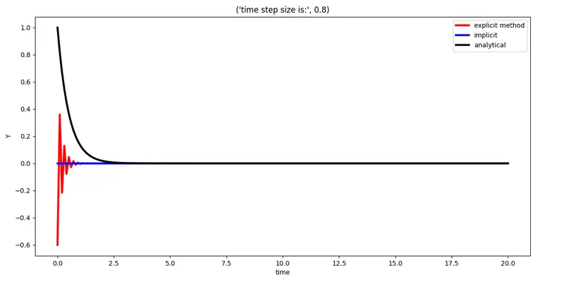
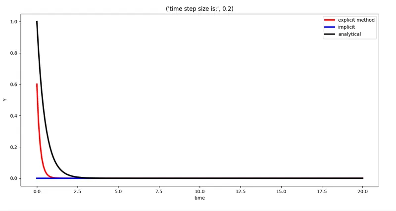
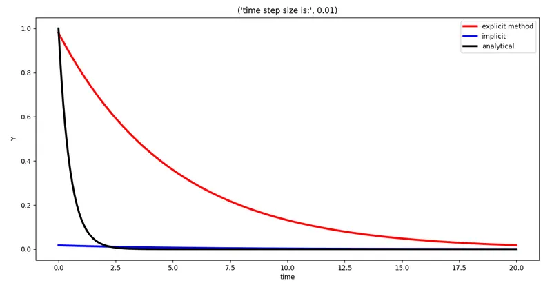
now by changing the time step we get the following plots 

Conclusion

1)The implicit method solution is not affected by time step at all,that means we can say that it is unconditionally stable in regard of which time step we choose.

2)explicit method solution is approaching the analytical solution with the value of decreasing time step value,but at the time step size 1 the solution is oscillating between -1 and 1,so if we use the time step greater than one than the explicit solution will blow up.

3)if the time step size is less than one than explicit method will also give stable solution for this ode.