Week 5.2 - Literature review: ODE Stability
REPORT OF LITERATURE REVIEW OF ODE STABILITY
Contents:
- When does a ODE become unstable?
- How does stability affect engineering simulations?
- Can stability condition be derived for all types of problems?
- Program on Python to show the ODE stability.
1.1 When does a ODE become unstable?
When a Solution to Ordinary differential equation is approached by iterative numerical methods, the absolute error between iterations gives us an idea about the stability criteria of the Solution. For stable Solution, the error between the iterations sholud decrease. the step size in the iterative method along with teh discrete point density in the domain of iteration plays a vital role in the Stability of the Solution
For the Stable solution the dt = time step size is less and the number of points in the domain is also should be large for stable system that is why appropiate selection of step size and grid density is very vital for stable equilibrium.
Courant number also plays an important role for system stabilty
The Courant number is a non-dimensional number named after the mathematician Richard Courant. The Courant number can be used in Computational Fluid Dynamics (CFD) simulations to evaluate the time step requirements of a transient simulation for a given mesh size and flow velocity and is linked to the Courant–Friedrichs–Lewy (CFL) stability condition of numerical schemes.
The Courant number formula is defined as
Where U indicates the flow velocity, Δt is a representative time step of the simulation and Δh the characteristic size of the mesh cell (in 1 dimension). For multi-dimensional problems, the condition can be evaluated as the sum in all directions, i.e.,
In a CFD simulation, the Courant number broadly indicates how much the information travels ( U ) across a computational grid cell ( Δh ) in a unit of time ( Δt ). If the Courant number is greater than one, it means that the information propagates through more than one grid cell at each time step, making the solution inaccurate and potentially leading to nonphysical results or divergence of the solution in certain integration schemes.
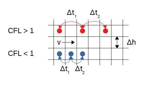
The Courant number plays an important role when running a transient CFD simulation, where we are interested in the variations of the flow field in time as well as in space. The physical time is discretised using a time step and the choice of time step has two main implications: one is related to the stability of the time discretisation scheme; the other is related to the physical meaning of the time step.
1.2 How does stability affect engineering simulations?
If the System is not stable the output or gained values must be unrealstic, there might be too much variation withe the actual experimental results. Such solutions are not acceptable and should not be trusted for futher study.
there are various stability criterion develped for particular type of Differentail equations
1.3 Can stability condition be derived for all types of problems?
For ODE system, stability analysis is divided into the following:
- Linear ODE Stability
- Stabilty of autonomous ODE system
- Non-linear stability systems.
- ODE stablity for Multivariable systems
To check the Stability criteria of particular ODE
`dy/dt = -1000y-e^-t`
Using Explicit numerical method, Solving the differential equation:
`(y^(i+1) - yi)/dt` = `-1000y^i-e^-t`
Using implicit numerical method:
`y^(i+1)` = `(y^i - e^-tdt)/(1+1000dt)`
Anaytical Solution:
`e^(-1000t)*(1-e^(999t))/999`
1.4 Python code To check the ODE stability:
"""
Explicit, Implicit and Anaytical euler Equations to check the ODE stability
"""
import math
import matplotlib.pyplot as plt
import numpy as np

def explicit_euler(T,dt):
	t = np.arange(0,T,dt)
	y = np.zeros(len(t))

	for i in range(1,len(t)):
		y[i] = y[i-1] + dt*(-1000*y[i-1]- np.exp(-t[i-1]))

	return [t,y]

def implicit_euler(T,dt):
	t = np.arange(0,T,dt)
	y = np.zeros(len(t))

	for i in range(1,len(t)):
		y[i] = (y[i-1]- np.exp(-t[i-1])*dt)/(1 + 1000*dt)

	return [t,y]

def analytical_euler(T,dt):
	t = np.arange(0,T,dt)
	y = np.zeros(len(t))

	for i in range(1,len(t)):
		y[i] = (np.exp(-1000*t[i])*(1-np.exp((1000-1)*t[i])))/(1000-1)

	return [t,y]

T = 0.1
dt = 1.5e-3

t,y_explicit = explicit_euler(T,dt)
t,y_implicit = implicit_euler(T,dt)
t,y_analytical = analytical_euler(T,dt)

plt.plot(t,y_explicit,'--',color= 'green')
plt.plot(t,y_implicit,'-.',color = 'blue')
plt.plot(t,y_analytical,color = 'red')
plt.legend(['Explicit','Implicit','Analytical'])
plt.show()
Output we got from this program:
dt = 1e-2
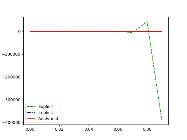
In the above graph we can see that there is divergence occurs in the Explicit Differencing scheme. and Implicit scheme is converged with the Anyalytical scheme of differencing.
dt = 1e-3
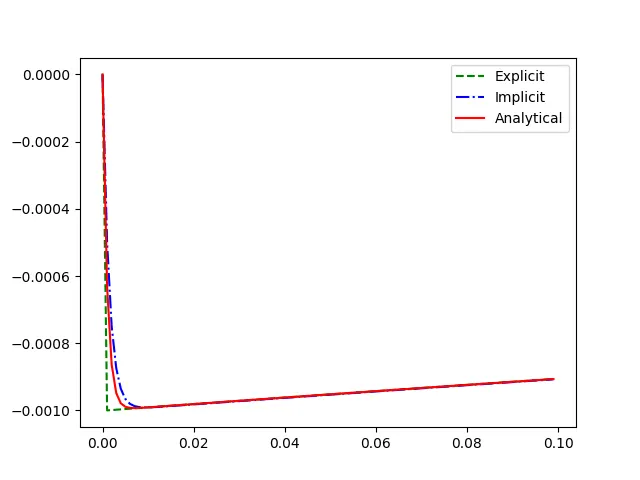
In this graph Explicit scheme are getting converged as compared to the previous graph and th Implciit scheme is also try to converged it more as compared to the explicit scheme.
dt = 1e-4
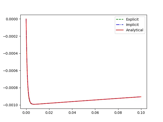
In this both the Explicit and Implicit Scheme is converged with the Analytical Solution Scheme and its us Accurate results with the Analytical Solution.
dt = 1.5e-3
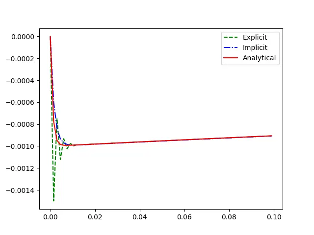
When dt = 1.5e-3 the System starts oscillating or system becomes unstable as you seen in the Above graph at the time step 0.01s after that it started to converge the Solution.