Week 5.2 - Literature review: ODE Stability

ODE Stability:

Aim:

To understand when a Ordinary Differential Equation solved using Explicit method, becomes unstable.

And understand its effect on engineering simulations.

Description:

In mathematics, an ordinary differential equation (ODE) is a differential equation containing one or more functions of one independent variable and the derivatives of those functions. The term ordinary is used in contrast with the term partial differential equation which may be with respect to more than one independent variable.

These differential equations results mostly when we try to model a physical process. In our case we get the differential equations, when we try to solve conservation equations. When the analytical methods are not available to solve a ODE, we solve them using numerical methods. These numerical methods are approximate methods, but serve the engineering purposes.

These numerical methods are not straight forward and will not work always (example: stability), if the required conditions are not met.

We will see when a ODE becomes unstable.

Let the differential equations be of the form:

`f(t) = (dy)/(dt) = -1000y - exp(-t)`

initial conditions are

y = 0 at t = 0

Explicit Method (Euler forward differencing with time):

`(y^(i+1) - y^(i))/dt = -1000y^i - e^(-t)`

`y^(i+1) = (-1000y^i - e^(-t))*dt + y^(i)`

Implicit Method (Euler forward differencing with time):

`(y^(i+1) - y^(i))/dt = -1000y^(i+1) - e^(-t)`

`y^(i+1) = (y^(i) - e^(-t)*dt)/(1 + 1000*dt)`

Analytical Method:

`y = e^(-1000*t)*(1-e^(999*t))/999`

Code:

Python code used for plotting graphs

"""
demonstration of stability of ode
"""

import numpy as np
import matplotlib.pyplot as plt

def explicit_euler(total_t, dt):
	t  = np.arange(0, total_t, dt)
	y = np.zeros(len(t))

	for i in range (1,len(t)):
		y[i] = y[i-1] + dt*(-1000*y[i-1] - np.exp(-t[i-1]))

	return [t,y]
def implicit_euler(total_t, dt):
	t = np.arange(0,total_t,dt)
	y = np.zeros(len(t))

	for i in range (1,len(t)):
		y[i] = (y[i-1] - np.exp(-t[i-1])*dt)/(1 + 1000*dt)

	return [t,y]

def analytical(total_t, dt):
	t = np.arange(0,total_t,dt)
	y = np.zeros(len(t))

	for i in range (1,len(t)):
		y[i] = np.exp(-1000*t[i])*(1 - np.exp(999*t[i]))/999

	return y

total_t = 0.1
dt = 1.5e-4
t, y_explicit = explicit_euler(total_t,dt)
t, y_implicit = implicit_euler(total_t,dt)
y_analytical = analytical(total_t,dt)
plt.plot(t, y_explicit)
plt.plot(t, y_implicit)
plt.plot(t, y_analytical)
plt.legend(['Explicit','Implicit','Analytical'])
plt.grid()
plt.show()

Plots:

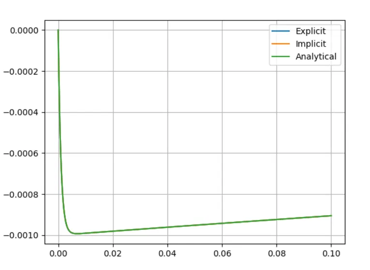
When dt = 1e-5

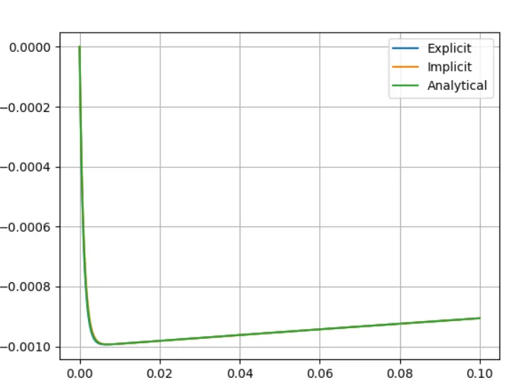
When dt = 1e-4

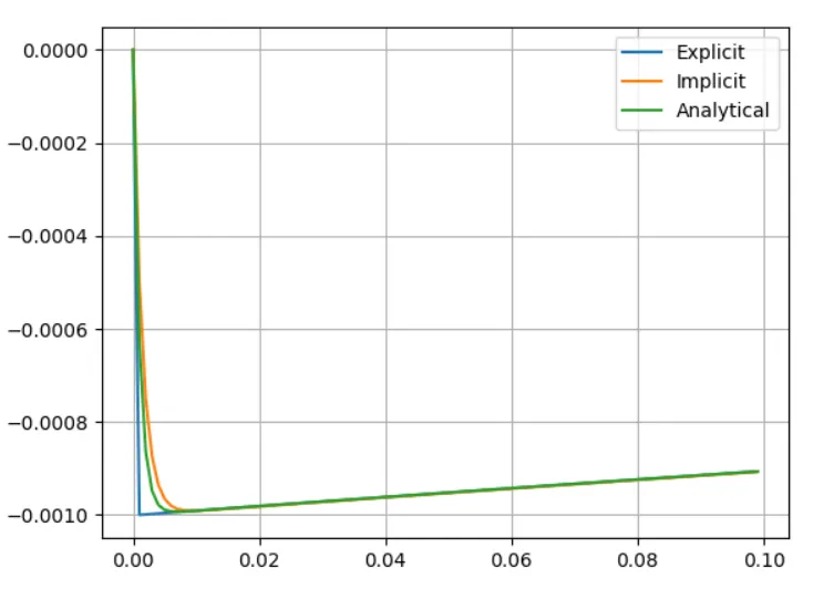
When dt = 1e-3

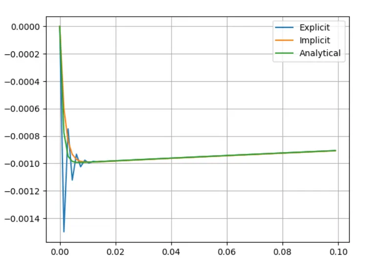
When dt = 1.5e-3

When dt = 1.9e-3

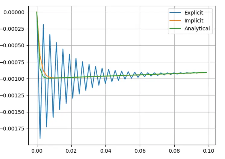
Comments:

From the above plots we can see that as we increase the time step size:

a. Analytical solution has no effect (As it is not calculated based on time step).

b. Implicit Method solution error is increasing but giving consistent or relevant solution.

c. Explicit method solution is giving good results at low time step value. Error is increasing as we increase the time step value. But beyond a certain value of time step, the solution is becoming unstable and gives physically irrelevant results. The solution becomes unstable and blow as the simulation progresses, when the error increases for each and every time step.

We can make use of this fact that the error should not increase as simulation progresses and derive a stability criterion. But we cannot derive this criterion for all problems. This is possible only for linear differential equations. But non-linear differential equations also becomes unstable arround the same value of time step, as given by the analysis for linear differential equations.

In engineering simulations, we avoid unstable solutions as it gives meaningless results. For this reason in Explicit method, we need to use small value of step size which increases the computational cost and time. As implicit methods don't have the problem of stability, we can use any step size based on the required accuracy of solution.