Challenge

Week 5.1 - Mid term project - Solving the steady and unsteady 2D heat conduction problem

AAkhilesh Gorilla26 May 2021

MATLAB

AIM: To write a program for solving the steady and unsteady 2D heat conduction problem.

OBJECTIVE:

Steady state analysis & Transient State Analysis.
Solve the 2D heat conduction equation by using the point iterative techniques.
Implement the following methods for solving implicit equations.

1. Jacobi

2. Gauss-seidel

3. Successive over-relaxation

absolute error criteria is 1e-4.

INPUTS:

Top Boundary = 600 K

Bottom Boundary = 900 K

Left Boundary = 400 K

Right Boundary = 800 K

EXPLANATION AND THEORY:

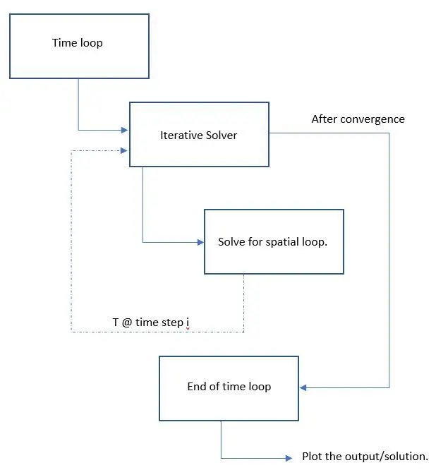
ALGORITHM USED FOR THIS CODE:

STEADY STATE CASE:

a) JACOBI METHOD:

For the steady state 2D conduction equation given by: ∂^2T/∂x^2 + ∂^2T/∂y^2 =0.

The solution using jacobi method can be written as,

T_pk+1 = Δy^2(T_Lk + T_Rk) + Δx2(T_Tk + T_Bk) / 2(Δx^2+Δy^2)

This equation is iterated with the help of neighbouring values of the previous iteration until the error between two consucutive iterations comes down below the set tolerance level. This method is called convergence.

k is the iteration number.

b) GAUSS-SEIDAL METHOD:

For the steady state 2D conduction equation given by: ∂^2T/∂x^2 + ∂^2T/∂y^2 =0.

The solution using Gauss seidel method can be written as,

T_pk+1 = Δy^2(T_Lk+1 + T_Rk) + Δx^2(T_Tk+1 + T_Bk) / 2(Δx^2+Δy^2)

This is similar toi Jacobi method but instead of considering the neighbouring values from previous iteration here the know values of the current iteration is taken into account and hence reaches faster convergence with lower number of iterations.

k is the iteration number

c) SOR METHOD:

For the steady state 2D conduction equation given by: ∂^2T/∂x^2 + ∂^2T/∂y^2 =0.

The solution using SOR method can be written as,

T_pk+1 = (1-ω) . T_pk + ω . Δy^2(T_Lk+1 + T_Rk) + Δx^2(T_Tk+1 + T_Bk) / 2(Δx^2+Δy^2)

TRANSIENT CASE:

1. EXPLICIT SCHEME:

For the transient case along with iteration number there comes into consideration the variable with respect to time, which is time step size and number of time steps. For the steady state 2D conduction equation given by: ∂T/∂t = α . (∂^2T/∂x^2 + ∂^2T/∂y^2)

The explicit solution can be wtitten as,

T_pn+1-T_pn/Δt = α . ( T_L- 2 T_P+ T_R/Δx^2 + T_T- 2 T_P+ T_B/Δy^2 )

hence, this equation can be directly solved by looping over the spatial grid for all the grid points. Here, after rearranging and simplifying we get two constants and that are called as the CFL numbers which are defined as follows:

K₁= α . Δt/Δx^2 and K₂= α . Δt/Δy^2

These numbers are to be kept less that 0.5 in order for the solution to converge and produce meaningful results. hence it depends on the thermal diffusion coefficient, time step size and grid spacing size.

2. IMPICIT SCHEME:

Again the methods used for steady state simulation can be used to solve the equation iteratively.

a) JACOBI METHOD:

The solution equation after simplifying can be written as a set of following equations:

K₁= α . Δt/Δx^2 and K₂= α . Δt/Δy^2

term1 = 1/ 1 + 2K₁ + 2K₂and term2 = K₁. term1 and term3 = K₁ . term1

The tempreature at time step (n+1) can be calculated from the time step values and n and n+1 using:

T_pn+1 = term1 . T_pn + term2 . ( T_L + T_R)^n+1 + term3 . ( T_T + T_B)^n+1

All the values are considered from the previous iteration.

b) GAUSS-SEIDAL METHOD:

The solution equation after simplifying can be written as a set of following equations:

K₁= α . Δt/Δx^2 and K₂= α . Δt/Δy^2

term1 = 1/ 1 + 2K₁ + 2K₂and term2 = K₁. term1 and term3 = K₁ . term1

The tempreature at time step (n+1) can be calculated from the time step values and n and n+1 using:

T_pn+1 = term1 . T_pn + term2 . ( T_L + T_R)^n+1 + term3 . ( T_T + T_B)^n+1

Here known values are considered from the current iteration.

c) SOR METHOD:

The solution equation after simplifying can be written as a set of following equations:

K₁= α . Δt/Δx^2 and K₂= α . Δt/Δy^2

term1 = 1/ 1 + 2K₁ + 2K₂and term2 = K₁. term1 and term3 = K₁ . term1

The tempreature at time step (n+1) can be calculated from the time step values and n and n+1 using:

T_pn+1 =(1-ω) . T_p + ω( term1 . T_pn + term2 . ( T_L + T_R)^n+1 + term3 . ( T_T + T_B)^n+1)

MATLAB CODE:

FOR STEADY STATE CASE:

clear all
close all
clc
nx=10;
ny=10;
t=ones(nx,ny);
t(1,1:ny)=600;
method=0;
t(1:nx,1)=400;
t(1:nx,ny)=800;
t(nx,1:ny)=900;
t(1,1)=500;
t(10,1)=650;
t(1,10)=700;
t(10,10)=850;
t(2:nx-1,2:ny-1)=300;
x=linspace(0,1,nx);
y=linspace(0,1,ny);
dx= 1/(nx-1);
dy=1/(ny-1);
[xx yy]=meshgrid(x,y);
k=(2*(dx^2+dy^2)/((dx^2)*(dy^2)));
error=9e9;
tol=1e-4;
told1=t;
told2=t;
told3=t;
% t2=t;
tinitial=t;
j_iter=1;
gs_iter=1;
sor_iter=1;
w=0;
method=input('Enter method number 1.Jacobi 2.Gauss Seidel 3.SOR')
%Jacobi
if (method==1)
while error>tol

for i=2:nx-1
 for j=2:ny-1
 term1= (told1(i-1,j)+told1(i+1,j))/(dx^2);
 term2= (told1(i,j-1)+told1(i,j+1))/(dy^2);
 t(i,j)=(term1+term2)/k ;
 end
end
a = ((t-told1))
b=max(max(a))
error=b
told1=t;
j_iter=j_iter+1;
end
contourf(x,y,t,'showtext','on')
colormap(jet)
colorbar
set(gca,'YDIR','reverse')
xlabel('X axis')
ylabel('Y axis')
title(sprintf('2D steady state analysis (Jacobi) for %d number of iterations ',j_iter))
pause(0.02)
end
%Gauss Seidel
if(method==2)
 while error>tol

for i=2:nx-1
 for j=2:ny-1
 term1= (t(i-1,j)+told2(i+1,j))/(dx^2);
 term2= (t(i,j-1)+told2(i,j+1))/(dy^2);
 t(i,j)=(term1+term2)/k ;
 end
end
a = ((t-told2))
b=max(max(a))
error=b
told2=t;
gs_iter=gs_iter+1;
end
contourf(x,y,t,'showtext','on')
colormap(jet)
colorbar
set(gca,'YDIR','reverse')
xlabel('X axis')
ylabel('Y axis')
title(sprintf('2D steady state analysis (Gauss Seidel) for %d number of iterations ',gs_iter))
pause(0.02)
end
% Successive Over-relaxation
if(method==3)
 w=input('Enter omega value >1 for succesive over relaxation')
 while error>tol

for i=2:nx-1
 for j=2:ny-1
 term1= (t(i-1,j)+told3(i+1,j))/(dx^2);
 term2= (t(i,j-1)+told3(i,j+1))/(dy^2);
 t(i,j)=(term1+term2)/k ;
 t(i,j)=(1-w)*told3(i,j) + w.*t(i,j) ;
 end
end
a = abs((t-told3))
b=max(max(a))
error=b
told3=t;
sor_iter=sor_iter+1;
end
contourf(x,y,t,'showtext','on')
colormap(jet)
colorbar
set(gca,'YDIR','reverse')
xlabel('X axis')
ylabel('Y axis')
title(sprintf('2D steady state analysis (SOR) for %d number of iterations ',sor_iter))
pause(0.02)
end

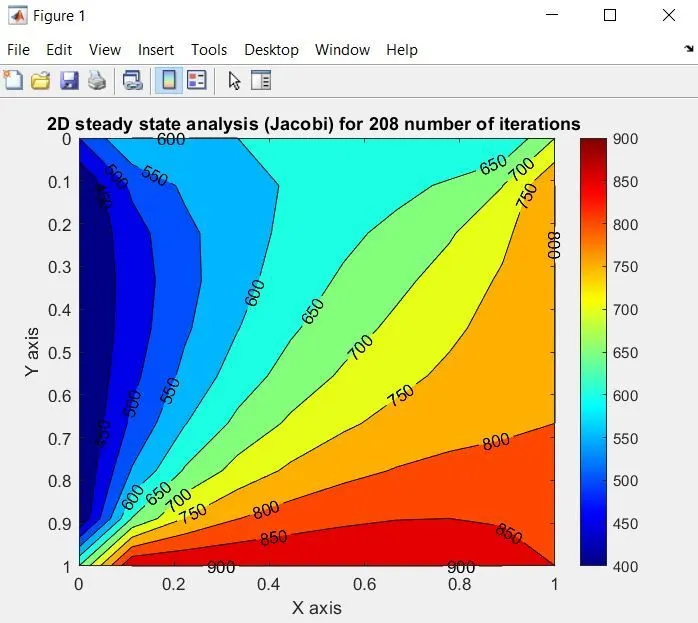
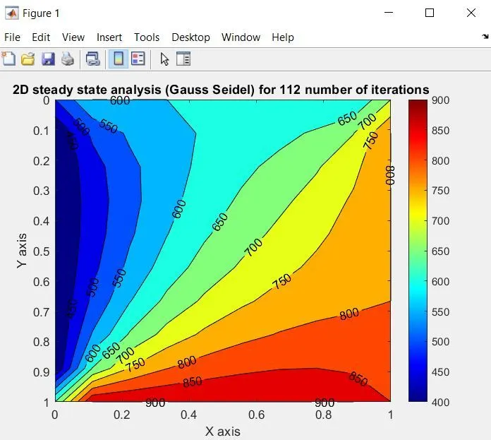
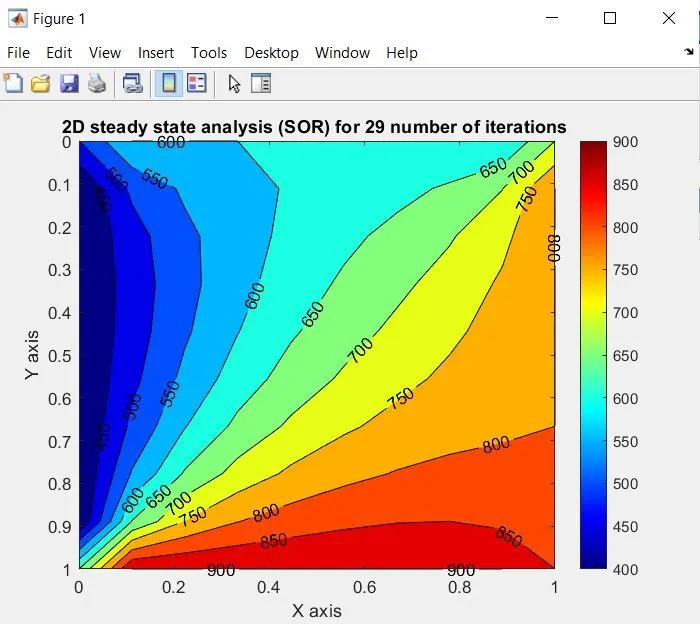
RESULTS FOR STEADY STATE CASE:

i) JACOBI:

ii) GAUSS SEIDAL:

iii) SUCCESSIVE OVER-RELAXATION:

FOR TRANSIENT CONDITION:

clear all
close all
clc
% To create a 10x10 matrix or domain of study with given boundary condition
nx=10;
ny=10;
t=ones(nx,ny);
t(1,1:ny)=600;
method=0;
t(1:nx,1)=400;
t(1:nx,ny)=800;
t(nx,1:ny)=900;
t(1,1)=500;
t(10,1)=650;
t(1,10)=700;
t(10,10)=850;
t(2:nx-1,2:ny-1)=300;
x=linspace(0,1,nx);
y=linspace(0,1,ny);
dx= 1/(nx-1);
dy=1/(ny-1);
[xx yy]=meshgrid(x,y);
% k=(2*(dx^2+dy^2)/((dx^2)*(dy^2)));
error=9e9;
tol=1e-4;
told=t;
told2=t;
tp=t;
told3=t;
% t2=t;
tinitial=t;
j_iter=1;
gs_iter=1;
sor_iter=1;
w=0;
a1=1.5;
t_tot=10;
dt=2
nt=t_tot/dt;
%nt=30;
k=a1*dt/(dx^2);
%CFL number to check for stability condition
CFL=a1*dt/(dx^2);
method=input('enter method 1.explicit 2.implicit jacobi 3.implicit Gauss seidel 4. implicit SOR');
if(method==1)
 a1=0.02;
t_tot=10;
dt=0.1;
nt=t_tot/dt;
%nt=30;
k=a1*dt/(dx^2);
CFL=a1*dt/(dx^2);
% Explicit scheme

for o=1:nt
 for i=2:nx-1

 for j=2:ny-1

 term1= (told(i-1,j)-(2*told(i,j))+told(i+1,j));
 term2= (told(i,j-1)-(2*told(i,j))+told(i,j+1));
 t(i,j)=told(i,j)+k*(term1+term2) ;

 end
 end

error =max(max(abs(told-t)));
told=t;
end
% To plot contour (same code for all cases)
contourf(x,y,t,'showtext','on')
colormap(jet)
colorbar
set(gca,'YDIR','reverse')
xlabel('X axis')
ylabel('Y axis')
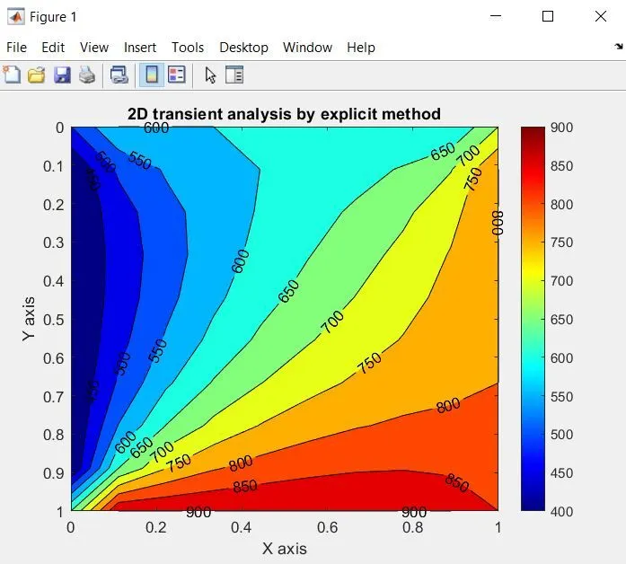
title(sprintf('2D transient analysis by explicit method'))
pause(0.02)
end
%Implicit scheme
if (method==2)


 % Time step iteration (for all cases)
 for o=1:nt
 while error>tol
 % Space step iteration (for all cases )
for i=2:nx-1
 for j=2:ny-1
 term1=(1+(4*k))^-1;
 term2=k*term1;
 H=(told(i-1,j)+told(i+1,j));
 V=(told(i,j-1)+told(i,j+1));
 t(i,j)=(tp(i,j)*term1)+(H*term2)+(V*term2);
 end
end
a = abs((t-told))
b=max(max(a))
error=b
told=t;
j_iter=j_iter+1;
end
tp=told;
 end
 contourf(x,y,t,'showtext','on')
colormap(jet)
colorbar
set(gca,'YDIR','reverse')
xlabel('X axis')
ylabel('Y axis')
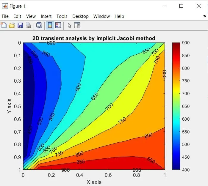
title(sprintf('2D transient analysis by implicit Jacobi method'))
pause(0.02)
end
% Gauss Seidel
if (method==3)

 for o=1:nt
 while error>tol

for i=2:nx-1
 for j=2:ny-1
 term1=(1+(4*k))^-1;
 term2=k*term1;
 H=(t(i-1,j)+told2(i+1,j));
 V=(t(i,j-1)+told2(i,j+1));
 t(i,j)=(tp(i,j)*term1)+(H*term2)+(V*term2);

 end
end
a = abs((t-told2))
b=max(max(a))
error=b
told2=t;
gs_iter=gs_iter+1;
end
tp=told;
 end
 contourf(x,y,t,'showtext','on')
colormap(jet)
colorbar
set(gca,'YDIR','reverse')
xlabel('X axis')
ylabel('Y axis')
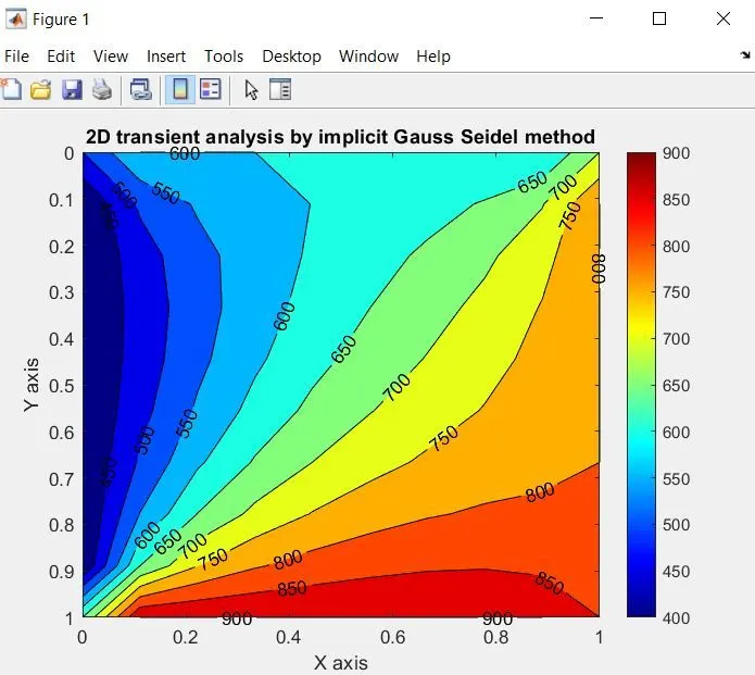
title(sprintf('2D transient analysis by implicit Gauss Seidel method'))
pause(0.02)
 end
%SOR
if (method==4)
 w=input('Enter omega value for succesive over relaxation')
 for o=1:nt
 while error>tol

for i=2:nx-1
 for j=2:ny-1
 term1=(1+(4*k))^-1;
 term2=k*term1;
 H=(t(i-1,j)+told3(i+1,j));
 V=(t(i,j-1)+told3(i,j+1));
 t(i,j)=(tp(i,j)*term1)+(H*term2)+(V*term2);
 t(i,j)=(1-w)*told3(i,j) + w.*t(i,j)
 end
end
a = abs((t-told3))
b=max(max(a))
error=b
told3=t;
sor_iter=sor_iter+1;
end
tp=told;
 end
 contourf(x,y,t,'showtext','on')
colormap(jet)
colorbar
set(gca,'YDIR','reverse')
xlabel('X axis')
ylabel('Y axis')
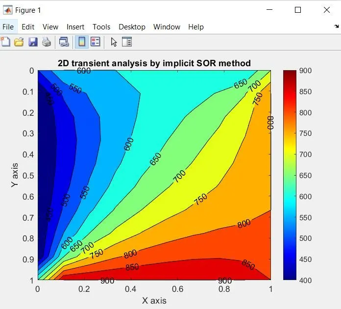
title(sprintf('2D transient analysis by implicit SOR method'))
pause(0.02)
end

RESULTS FOR TRANSIENT CONDITION:

a) EXPLICIT SCHEME: