Week 5.1 - Mid term project - Solving the steady and unsteady 2D heat conduction problem
Solving the steady and unsteady 2D heat conduction problem
Aim
Solve the 2D heat conduction equation by using the point iterative techniques for Steady & Transient State.
Description: -
Solving the 2D heat conduction equation by using the point iterative techniques for Steady & Transient State, using explicit and implicit schemes.
2-D Heat conduction equation
`(partial T)/(partial t) - alpha*((partial^2 T)/(partial x^2) + (partial^2 T)/(partial y^2) ) = 0`
in te above equation first term is Time derivative and second term is Spatial derivative. alpha is thermal diffusivity.
Steady-state: -
A system or a process is said to be a steady-state if the variables which define the behavior of the system or the process are unchanging in time. In continuous-time, this means that for those properties p of the system, the partial derivative with respect to time is zero and remains so.
`(partial T)/(partial t)= 0`
then the 2-D heat conduction equation becomes
`((partial^2 T)/(partial x^2) + (partial^2 T)/(partial y^2) ) = 0`
we have to discretize the above equation to get an approximate solution. the order above equation is 2 and we require 2nd order approximation so we have to apply a central differencing scheme to discretize.
after discretizing we get the final equation as
`T_(i,j)= (∆x^2 ∆y^2)/(2(∆x^2+∆y^2))*[(T_(i-1,j)+T_(i+1,j))/(∆x^2 )+(T_(i,j-1)+T_(i,j+1))/(∆y^2 )]`
Simply
`K =(2(∆x^2+∆y^2))/(∆x^2 ∆y^2)`
`T_(i,j)= (1/K)*[(T_L+T_R)/(∆x^2 )+(T_T+T_B)/(∆y^2 )]`
Transient state
A system is said to be in a transient state when a process variable or variables have been changed and the system has not yet reached a steady-state. The time taken for the circuit to change from one steady-state to another steady state is called the transient time.
`(partial^2 T)/(partialt^2 )= α((partial^2 T)/(partialx^2 )+(partial^2 T)/(partialy^2 ))`
n the processes of discretization of the above equation, we have to use forward differencing for time derivative and central differencing for space derivative.
after discretizing the final equation becomes
`T_(i,j)^(n+1)=T_(i,j)^n+(α∆t)/(∆x^2 ) (T_(i-1,j)-2T_(i,j)+T_(i+1,j) )^n+(α∆t)/(∆y^2 ) (T_(i,j-1)-2T_(i,j)+T_(i,j+1) )^n`
We have to use Explicit and Implicit schemes to solve Transient analysis.
Explicit scheme: -
in explicit we use n time step values to calculate values at n+1 time step i.e., we get coupled equations with R.H.S known to find L.H.S.
`T_P^(n+1) = T_P^n*(1-(2.K 1) - (2.K 2) ) + (K 1*(T_L^n +T_R^n)) + (K 2*(T_B^n+T_T^n))`
Implicit scheme: -
in implicit we use n time step vales to calculate values at n time step i.e., we get un-coupled equations with both R.H.S & L.H.S are un-known.
`T_P^(n+1) = T_P^n + K 1*(T_L^(n+1) - 2*T_P^(n+1) + T_R^(n+1)) + K 2 *(T_T^(n+1) - 2*T_P^(n+1) + T_B^(n+1))`
To solve implicit scheme we require iterative techniques they are.
- Jacobi Method :- `T_P^(n+1) = (T_P^n + K 1*(T_L^(n)+ T_R^n) + K 2*(T_T^(n) + T_B^n) ) / (1+2*K 1+2*K 2)`
- Gauss-Seidel Method :- `T_P^(n+1) = (T_P^n + K 1*(T_L^(n+1)+ T_R^(n)) + K 2*(T_T^(n+1) + T_B^(n)) ) / (1+2*K 1+2*K 2)`
- Successive Over Relaxation method :- `T_P^(n+1) = T_P^n*(1-omega) + omega*[(T_P^n + K 1*(T_L^(n+1)+ T_R^(n)) + K 2*(T_T^(n+1) + T_B^(n)) ) / (1+2*K 1+2*K 2)]` omega is a relaxation factor for SOR
Given data: -
- Top Boundary = 600 K
- Bottom Boundary = 900 K
- Left Boundary = 400 K
- Right Boundary = 800 K
- Error criteria = 1e-4
CFL number:
The courant number or CFL number is the fraction of the cell that the flow moves across in a time step.
`CFL = alpha*((Deltat)/(Deltax^2)+(Deltat)/(Deltay^2))<=0.5`
It measure of how much information c flow through a grid cell size dx & dy in a given time-step dt.
CFL condition is considered only for explicit solution not for implicit solution
Procedure: -
- Define the inputs length of domain along x & y-axis and specify number of divisions.
- do some calculations to find meshgrid,nx,ny,dx,dy,K.
- Specify boundary conditions.
- for Steady state equation by using space loop in convergence loop.
- for transient state create space loop in convergence loop & convergence loop in time loop for different schemes and methods.
- plot the results.
Steady-state:-
SS function programs:-
function steady_plot(xx,yy,T,itr)
% [x_x, y_y] = contourf(xx,yy,T);
% clabel(x_x,y_y);
contourf(xx,yy,T);
colormap(jet); colorbar
set(gca,'ydir','reverse')
xlabel('length of domain along X-axis'); ylabel('length of domain along Y-axis')
title_text1 = sprintf('Total  number of iterations taken to converge the solution is = %d iterations',itr);
title({'Transient 2 D heat conduction temperatute profile';title_text1})
pause(0.00003)
end
Main program:
% Steady state analysis
clear all; close all; clc

inputs = {'length of domain along x-axis';'length of domain along y-axis';'number of divisions along x-axis';'number of divisions along y-axis'};
dlgtitle = 'Spatial inputs';
dims = [1 50];
definput = {'1';'1';'30';'30'};
B  = inputdlg(inputs,dlgtitle,dims,definput);

%inputs
 L_x = str2double(B{1});                      % length of domain along x-axis
 L_y = str2double(B{2});                      % length of domain along y-axis
 nx = str2double(B{3}) ;                    % number of divisions along x-axis / columns
 ny = str2double(B{4});                    % number of divisions along y-axis / rows

x = linspace(0,L_x,nx);
y = linspace(0,L_y,ny);
[xx, yy] = meshgrid(x,y) ;
 T = 300*ones(ny,nx);         % creating mesh grid on domain
  % calculations
 dx = L_x/(nx-1);
 dy = L_y/(ny-1);
 K = 2*((dx^2+dy^2)/(dx^2*dy^2));
 %%
 %given boundry condiions
 T_t = 600;  T(1,:)    = T_t;                  % Top Boundary Temperature in K
 T_b = 900;  T(end,:)  = T_b;                  % Bottom Boundary Temperature in K
 T_l = 400;  T(:,1)    = T_l;                  % Left Boundary Temperature in K
 T_r = 800;  T(:,end)  = T_r;                  % Right Boundary Temperature in K

 % Assigning BC to corners
 T(1,1)     = (T_t+T_l)/2;
 T(1,end)   = (T_t+T_r)/2;
 T(end,end) = (T_b+T_r)/2;
 T(end,1)   = (T_l+T_b)/2;

 % creating a copy of u
 Told = T;
 Tcopy = T;
 error = 1;
 tolerance = 1e-4;

 %%
 tic
 itr = 0;
     while (error > tolerance)
         for i = 2:(ny-1)
             for j = 2:(nx-1)
                 T(i,j) = (1/K)*((Told(i,(j-1))+Told(i,(j+1)))/dx^2+(Told((i-1),j)+Told((i+1),j))/dy^2);
         end
     end
        error = max(max(abs(Told-T)));
        Told = T;
        itr = itr+1;
%steady_plot(xx,yy,T,itr)
     end
computation_time = toc;
contourf(xx,yy,T);
colormap(jet); colorbar
set(gca,'ydir','reverse')
xlabel('length of domain along X-axis'); ylabel('length of domain along Y-axis')
title_text1 = sprintf('Computation_time taken  to solve is = %0.6f seconds',computation_time);
title_text2 = sprintf('Total  number of iterations taken to converge the solution is = %d iterations',itr);
title({'Steady state 2 D heat conduction temperatute profile';title_text1;title_text2})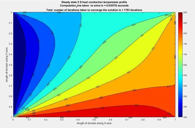
Transient Analysis:-
plot function program
function transient_plot(xx,yy,T,dx,dy,dt,nt,CFL,t,itr,computation_method)
%[x_x, y_y] = contourf(xx,yy,T)
%clabel(x_x,y_y);
contourf(xx,yy,T)
colormap(jet); colorbar
set(gca,'ydir','reverse')
xlabel('length of domain along X-axis'); ylabel('length of domain along Y-axis')
title_text1 = sprintf('dx = %0.5f, dy = %0.5f, dt = %0.5f,  nt = %d, CFL = %0.5f, t = %0.5f sec',dx,dy,dt,nt,CFL,t);
title_text2 = sprintf('Total  number of iterations taken to converge the solution is = %d iterations',itr);
title({'Transient 2 D heat conduction temperatute profile';computation_method;title_text1;title_text2})
pause(0.00003)
end
% Transient analysis
clear all; close all; clc
inputs = {'length of domain along x-axis';'length of domain along y-axis';
'number of divisions along x-axis';'number of divisions along y-axis';
'Thermal diffucivity';'time step =';'number of time steps'};
dlgtitle = 'Spatial inputs & constants';
dims = [1 50];
definput = {'1';'1';'30';'30';'1.4';'0.0001';'1500'};
B = inputdlg(inputs,dlgtitle,dims,definput);
%inputs
L_x = str2double(B{1}); % length of domain along x-axis
L_y = str2double(B{2}); % length of domain along y-axis
nx = str2double(B{3}) ; % number of divisions along x-axis / columns
ny = str2double(B{4}); % number of divisions along y-axis / rows
alpha =str2double(B{5});
%t = str2double(B{6});
dt = str2double(B{6});
nt = str2double(B{7});
x = linspace(0,L_x,nx);
y = linspace(0,L_y,ny);
[xx, yy] = meshgrid(x,y) ;
T = 300*ones(ny,nx); % creating mesh grid on domain
% calculations
dx = L_x/(nx-1);
dy = L_y/(ny-1);
%dt = t/nt;
t = dt*nt;
K1 = alpha*dt/(dx^2);
K2 = alpha*dt/(dy^2);
CFL = K1+K2;
%%
%given boundry condiions
T_t = 600; T(1,:) = T_t; % Top Boundary Temperature in K
T_b = 900; T(end,:) = T_b; % Bottom Boundary Temperature in K
T_l = 400; T(:,1) = T_l; % Left Boundary Temperature in K
T_r = 800; T(:,end) = T_r; % Right Boundary Temperature in K
% Assigning BC to corners
T(1,1) = (T_t+T_l)/2;
T(1,end) = (T_t+T_r)/2;
T(end,end) = (T_b+T_r)/2;
T(end,1) = (T_l+T_b)/2;
%%
% creating a copy of u
Told = T;
T_pre = T;
error = 1;
tolerance = 1e-4;
%%
%%
D = inputdlg({'1) Explicit 2) Implicit'},'Enter solution_method = ',[1 50],{'1'});
solution_method =str2double(string(D{1}));
tic
itr = 0;
if solution_method == 1
computation_method = 'Transient Explicit computation method';
for k = 1:nt
for i = 2:(ny-1)
for j = 2:(nx-1)
term1 = K1*(Told(i,(j-1))-2*Told(i,j)+Told(i,(j+1)));
term2 = K2*(Told((i-1),j)-2*Told(i,j)+Told((i+1),j));
T(i,j) = Told(i,j)+term1+term2;
end
end
Told = T;
T_pre = T;
itr = itr+1;
% transient_plot(xx,yy,T,dx,dy,dt,nt,CFL,t,itr,computation_method)
end
elseif solution_method ==2
C = inputdlg({'1) Jacobi computation method /n 2) Gauss siedel computation method /n 3) SOR computation method'},'Enter computation method number = ',[1 50],{'2'});
iterative_solver = str2double(string(C{1}));
%%
if iterative_solver == 1
computation_method = 'Transient Implicit Jacobi computation method';
for k = 1:nt
error = 1;
while (error > tolerance)
for i = 2:(ny-1)
for j = 2:(nx-1)
T(i,j) = (1/(1+2*K1+2*K2))*(T_pre(i,j)+K1*(Told(i,(j-1))+Told(i,(j+1)))+K2*(Told((i-1),j)+Told((i+1),j)));
end
end
error = max(max(abs(Told-T)));
Told = T;
itr = itr+1;
% transient_plot(xx,yy,T,dx,dy,dt,nt,CFL,t,itr,computation_method)
end
T_pre = T;
end
elseif iterative_solver == 2
computation_method = 'Transient Implicit Gauss siedel computation method';
for k = 1:nt
error = 1;
while (error > tolerance)
for i = 2:(ny-1)
for j = 2:(nx-1)
T(i,j) = (1/(1+2*K1+2*K2))*(T_pre(i,j)+K1*(T(i,(j-1))+Told(i,(j+1)))+K2*(T((i-1),j)+Told((i+1),j)));
end
end
error = max(max(abs(Told-T)));
Told = T;
itr = itr+1;
%transient_plot(xx,yy,T,dx,dy,dt,nt,CFL,t,itr,computation_method)
end
T_pre = T;
end
elseif iterative_solver == 3
computation_method = 'Transient Implicit SOR computation method';
w = str2double(inputdlg({'Omega = '},'input',[1 50],{'1.05'}));
for k = 1:nt
error = 1;
while (error > tolerance)
for i = 2:(ny-1)
for j = 2:(nx-1)
T_G(i,j) = (1/(1+2*K1+2*K2))*(T_pre(i,j)+K1*(T(i,(j-1))+Told(i,(j+1)))+K2*(T((i-1),j)+Told((i+1),j)));
T(i,j) = Told(i,j)*(1-w)+w*T_G(i,j);
end
end
error = max(max(abs(Told-T)));
Told = T;
itr = itr+1;
% transient_plot(xx,yy,T,dx,dy,dt,nt,CFL,t,itr,computation_method)
end
T_pre = T;
end
end
end
computation_time = toc;
%%
%%
[x_x, y_y] = contourf(xx,yy,T);
clabel(x_x,y_y); colormap(jet); colorbar
set(gca,'ydir','reverse')
xlabel('length of domain along X-axis'); ylabel('length of domain along Y-axis')
title_text0 = sprintf('dx = %0.5f, dy = %0.5f, dt = %0.5f, nt = %d, CFL = %0.5f, t = %0.5f sec',dx,dy,dt,nt,CFL,t);
title_text1 = sprintf('Computation_time taken to solve is = %0.3f seconds',computation_time);
title_text2 = sprintf('Total number of iterations taken to converge the solution is = %d iterations',itr);
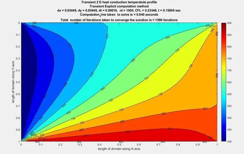
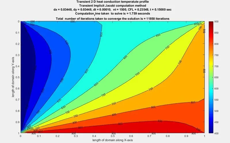
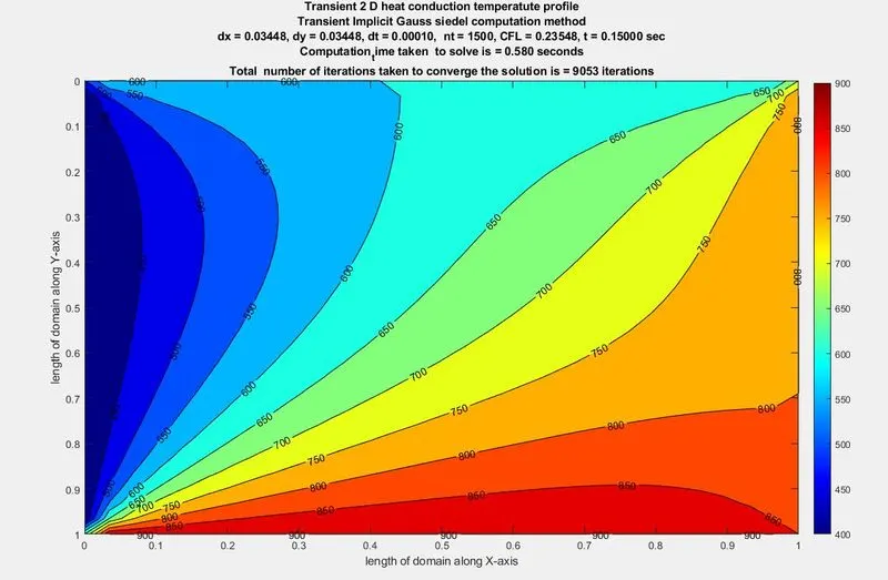
title({'Transient 2 D heat conduction temperatute profile';computation_method;title_text0;title_text1;title_text2})
%%
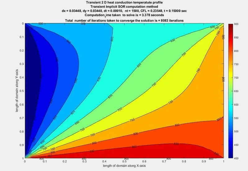
Conclusion: -
Steady-state analysis: -
To solve steady-state equations implicit method is preferred.
| Iterations | |
| Steady-state solver | 1783 |
Transient state analysis: -
| Iterations | |
| Transient Explicit | 1500 |
| Transient implicit Jacobi computation method | 11850 |
| Transient implicit Gauss Siedel computation method | 9053 |
| Transient implicit SOR computation method | 8083 |
SOR < Gauss <Jacobi